Module: Clustering Stability#
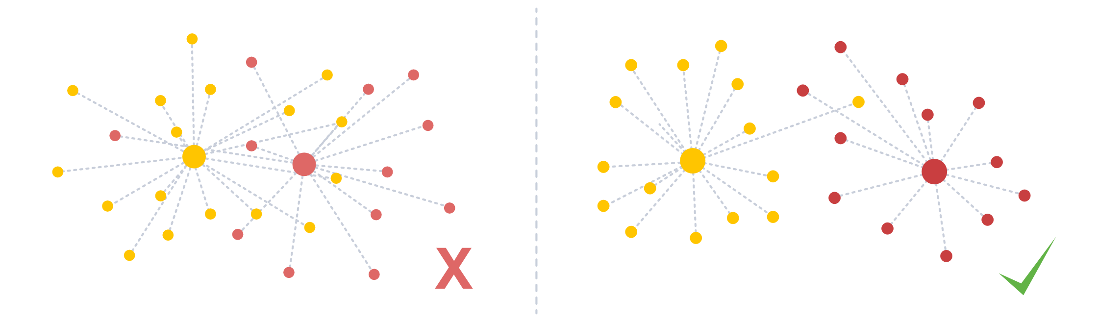
When analyzing (spatial) transcriptomics data, cells are typically clustered into cell types based on their RNA expression. If the segmentation of a spatial transcriptomics dataset went well, we would assume that this clustering is somewhat stable, even if we only cluster on parts of the data. The clustering stability (cs) module includes some functions to apply clustering and assess its robustness. The figure below shows a bad clustering (lots of overlap) vs. a good clustering.
To follow along with this tutorial, you can download the data from here.
[1]:
%load_ext autoreload
%autoreload 2
[21]:
import importlib
from pathlib import Path

import anndata as ad
import matplotlib.pyplot as plt
import pandas as pd
import scanpy as sc
import seaborn as sns
import spatialdata as sd
import spatialdata_plot  # noqa: F401

import segtraq
[3]:
# example datasets on which we can compare performance
st_bidcell = segtraq.SegTraQ(
    sd.read_zarr("../../data/xenium_5K_data/bidcell.zarr"),
    images_key="image",
    points_background_id=0,
    tables_centroid_x_key="centroid_x",
    tables_centroid_y_key="centroid_y",
)

st_segger = segtraq.SegTraQ(
    sd.read_zarr("../../data/xenium_5K_data/segger.zarr"),
    images_key="image",
    tables_centroid_x_key="cell_centroid_x",
    tables_centroid_y_key="cell_centroid_y",
)

st_xenium = segtraq.SegTraQ(
    sd.read_zarr("../../data/xenium_5K_data/xenium.zarr"),
    images_key="image",
    tables_centroid_x_key="x_centroid",
    tables_centroid_y_key="x_centroid",
)

st_proseg2 = segtraq.SegTraQ(
    sd.read_zarr("../../data/xenium_5K_data/proseg2.zarr"),
    images_key="image",
    points_background_id=0,
    tables_area_key=None,
    tables_centroid_x_key="centroid_x",
    tables_centroid_y_key="centroid_x",
)

st_dict = {"bidcell": st_bidcell, "segger": st_segger, "xenium": st_xenium, "proseg2": st_proseg2}
no parent found for <ome_zarr.reader.Label object at 0x7fff85eab620>: None
no parent found for <ome_zarr.reader.Label object at 0x7fff85f33610>: None
no parent found for <ome_zarr.reader.Label object at 0x7fff7435ce10>: None
no parent found for <ome_zarr.reader.Label object at 0x7fff74316b10>: None
/g/huber/users/meyerben/notebooks/spatial_transcriptomics/SegTraQ/src/segtraq/SegTraQ.py:116: UserWarning: Missing 23 cell IDs in shapes: ['ipkoiika-1', 'ickihlob-1', 'icjcpgce-1', 'icaegooe-1', 'hlhfagon-1']... These cells are present in tables, but not in shapes. This might lead to inconsistencies in the spatialdata object.
  validate_spatialdata(
/g/huber/users/meyerben/notebooks/spatial_transcriptomics/SegTraQ/src/segtraq/utils.py:1346: UserWarning: Duplicate IDs detected in index 'cell_id' for shapes 'nucleus_boundaries'. Resetting and renaming index to `segtraq_id` to ensure uniqueness.
  nucleus_shapes = _ensure_index(
no parent found for <ome_zarr.reader.Label object at 0x7fff74315e00>: None
no parent found for <ome_zarr.reader.Label object at 0x7fff85d22570>: None
/g/huber/users/meyerben/notebooks/spatial_transcriptomics/SegTraQ/src/segtraq/utils.py:1346: UserWarning: Duplicate IDs detected in index 'cell_id' for shapes 'nucleus_boundaries'. Resetting and renaming index to `segtraq_id` to ensure uniqueness.
  nucleus_shapes = _ensure_index(
no parent found for <ome_zarr.reader.Label object at 0x7fff744d7bd0>: None
no parent found for <ome_zarr.reader.Label object at 0x7fff744d7f00>: None
no parent found for <ome_zarr.reader.Label object at 0x7fff744e5d50>: None
no parent found for <ome_zarr.reader.Label object at 0x7fff744e7950>: None
no parent found for <ome_zarr.reader.Label object at 0x7fff74367c50>: None
no parent found for <ome_zarr.reader.Label object at 0x7fff743654f0>: None
/g/huber/users/meyerben/notebooks/spatial_transcriptomics/SegTraQ/src/segtraq/SegTraQ.py:116: UserWarning: Missing 4 cell IDs in shapes: [np.int64(11273), np.int64(10307), np.int64(10308), np.int64(6870)]... These cells are present in tables, but not in shapes. This might lead to inconsistencies in the spatialdata object.
  validate_spatialdata(
/g/huber/users/meyerben/notebooks/spatial_transcriptomics/SegTraQ/src/segtraq/utils.py:1346: UserWarning: Duplicate IDs detected in index 'cell_id' for shapes 'nucleus_boundaries'. Resetting and renaming index to `segtraq_id` to ensure uniqueness.
  nucleus_shapes = _ensure_index(
/g/huber/users/meyerben/notebooks/spatial_transcriptomics/SegTraQ/src/segtraq/SegTraQ.py:116: RuntimeWarning: No area column specified for tables. Area will be automatically computed from shapes.
  validate_spatialdata(
Important: Normalization and Log-Transform#
Since the clustering depends on a PCA, it is important that you normalize and log-transform your data before running the clustering methods. The code snippets below show how to do that.
[4]:
adata = st_dict["proseg2"].sdata.tables["table"]
adata.X[:5, :5].toarray()
[4]:
array([[ 3, 21,  4,  1,  7],
       [ 0,  1,  0,  1,  0],
       [ 2,  0,  0,  0,  0],
       [ 0,  4,  3,  3,  3],
       [ 0,  1,  0,  0,  0]])
[5]:
# preprocessing
for st in st_dict.values():
    # removing control transcripts
    st.filter_control_and_low_quality_transcripts()

    adata = st.sdata.tables["table"]
    adata.layers["counts"] = adata.X.copy()
    # normalizing and log-transforming the counts
    sc.pp.normalize_total(adata, inplace=True)
    sc.pp.log1p(adata)
    # computing a PCA and neighbors
    sc.pp.pca(adata)
    sc.pp.neighbors(adata)
/scratch/jobs/51410026/ipykernel_724080/4112654336.py:7: ImplicitModificationWarning: Setting element `.layers['counts']` of view, initializing view as actual.
  adata.layers["counts"] = adata.X.copy()
/scratch/jobs/51410026/ipykernel_724080/4112654336.py:9: UserWarning: Some cells have zero counts
  sc.pp.normalize_total(adata, inplace=True)
/g/huber/users/meyerben/notebooks/spatial_transcriptomics/SegTraQ/.venv/lib/python3.13/site-packages/tqdm/auto.py:21: TqdmWarning: IProgress not found. Please update jupyter and ipywidgets. See https://ipywidgets.readthedocs.io/en/stable/user_install.html
  from .autonotebook import tqdm as notebook_tqdm
/scratch/jobs/51410026/ipykernel_724080/4112654336.py:9: UserWarning: Some cells have zero counts
  sc.pp.normalize_total(adata, inplace=True)
/scratch/jobs/51410026/ipykernel_724080/4112654336.py:9: UserWarning: Some cells have zero counts
  sc.pp.normalize_total(adata, inplace=True)
/scratch/jobs/51410026/ipykernel_724080/4112654336.py:7: ImplicitModificationWarning: Setting element `.layers['counts']` of view, initializing view as actual.
  adata.layers["counts"] = adata.X.copy()
/scratch/jobs/51410026/ipykernel_724080/4112654336.py:9: UserWarning: Some cells have zero counts
  sc.pp.normalize_total(adata, inplace=True)
[6]:
adata = st_dict["proseg2"].sdata.tables["table"]
adata.X[:5, :5].toarray()
[6]:
array([[0.27639413, 1.1720397 , 0.3538137 , 0.10086061, 0.5555258 ],
       [0.        , 0.94614375, 0.        , 0.94614375, 0.        ],
       [3.9702919 , 0.        , 0.        , 0.        , 0.        ],
       [0.        , 0.9798287 , 0.8100409 , 0.8100409 , 0.8100409 ],
       [0.        , 0.79267675, 0.        , 0.        , 0.        ]],
      dtype=float32)
Note that we now have normalized and transformed counts, so we can move on to the clustering stability metrics.
The problem#
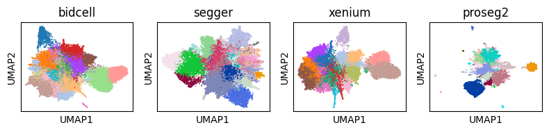
Segmentation hugely affects downstream analysis in spatial transcriptomics datasets. For example, let’s consider the UMAPs of four different segmentations. You can see below that they differ substantially.
[7]:
fig, axs = plt.subplots(1, 4, figsize=(8, 2))

# Flatten axs in case of single row/column
axs = axs.flatten()

for i, (method, st) in enumerate(st_dict.items()):
    # here, we do not want to alter the original data, so we create a deep copy
    sdata = st.sdata
    adata = sd.deepcopy(sdata.tables["table"])
    sc.tl.umap(adata)
    sc.tl.leiden(adata, flavor="igraph", n_iterations=2)

    sc.pl.umap(
        adata,
        color="leiden",
        ax=axs[i],
        show=False,
        title=method,
        legend_loc=None,
    )

plt.tight_layout()
plt.show()
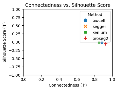
Cluster Connectedness#
The cluster connectedness (CC) is a measure that looks at the compactness of clusters. To compute it, we use the neighborhood graph we computed with scanpy earlier. The connectedness then iterates over all cells and computes the number of neighbors with the same cluster assignment and divides it by the number of total neighbors.
[8]:
ccs = {}
for method, st in st_dict.items():
    ccs[method] = st.cs.cluster_connectedness(use_weights=True, leiden_kwargs={"flavor": "igraph"})
ccs
[8]:
{'bidcell': 0.8756779533948085,
 'segger': 0.8464009069644749,
 'xenium': 0.854418260541604,
 'proseg2': 0.9190497059528142}
Silhouette Score#
A slightly more elaborate metric is the silhouette score. It measures how similar an object is to its own cluster (cohesion) compared to other clusters (separation). Values range from −1 to +1, where a high value indicates that the object is well matched to its own cluster and poorly matched to neighboring clusters.
We compute this metric for Leiden clustering at different resolutions and report the best one.
[9]:
silhouette_scores = {}
for method, st in st_dict.items():
    silhouette_scores[method] = st.cs.silhouette_score(leiden_kwargs={"flavor": "igraph"})
silhouette_scores
[9]:
{'bidcell': -0.0073308683931827545,
 'segger': -0.015781568363308907,
 'xenium': -0.00674070417881012,
 'proseg2': -0.057001955807209015}
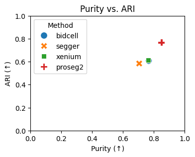
Purity#
Another way to assess cluster stability is to cluster only on a subset of all cells. For example, if we randomly select 63% (\(1 - e^{-1}\)) of cells and then perform Leiden clustering on those, will our cells typically get assigned to the same cluster or to different ones?
One way to assess this is by comparing the purity between two clusterings. For every cluster in clustering 1, we check how many other clusters it contains in clustering 2.
A purity value of 1 means that the clusters are completely pure, whereas a value closer to 0 means that they are more mixed.
We randomly select 63% of cells, perform clustering on them, and do this five times, to obtain five different clusterings. Then we compare them using the purity score.
Note: this method will recompute the PCA based on a subset of features. If you will be using the PCA in the anndata later, you should recompute it on the whole data.
[10]:
purities = {}
for method, st in st_dict.items():
    purities[method] = st.cs.purity(leiden_kwargs={"flavor": "igraph"})
purities
[10]:
{'bidcell': 0.7258176345941887,
 'segger': 0.736952447546779,
 'xenium': 0.753055778712793,
 'proseg2': 0.8413936954043493}
Adjusted Rand Index (ARI)#
The adjusted rand index (ARI) is another metric to determine the similarity of different clusterings (again, we create five clusterings based on random subsets of 63% of cells each). Just like the purity, its values range from 0 (no similarity, not a robust clustering) to 1 (exactly the same clusters, high robustness).
[11]:
aris = {}
for method, st in st_dict.items():
    aris[method] = st.cs.adjusted_rand_index(leiden_kwargs={"flavor": "igraph"})
aris
[11]:
{'bidcell': 0.5541955626905575,
 'segger': 0.6486254601137376,
 'xenium': 0.5978203745532411,
 'proseg2': 0.7354279239864419}
At the end, all of our metrics are stored in the spatialdata object.
[12]:
st_dict["proseg2"].sdata.tables["table"]
[12]:
AnnData object with n_obs × n_vars = 17885 × 5095
    obs: 'cell_id', 'centroid_x', 'centroid_y', 'centroid_z', 'volume', 'label_id', 'region', 'cell_area', 'leiden_subset_cells17885_res0.6_seed42', 'leiden_subset_cells17885_res0.8_seed42', 'leiden_subset_cells17885_res1.0_seed42', 'leiden_subset_cells11267_res1.0_seed0', 'leiden_subset_cells11267_res1.0_seed1', 'leiden_subset_cells11267_res1.0_seed2', 'leiden_subset_cells11267_res1.0_seed3', 'leiden_subset_cells11267_res1.0_seed4'
    uns: 'spatialdata_attrs', 'log1p', 'pca', 'neighbors', 'cluster_connectedness', 'silhouette_score', 'mean_purity', 'mean_ari'
    obsm: 'X_pca'
    varm: 'PCs'
    layers: 'X_estimated', 'counts'
    obsp: 'distances', 'connectivities'
Visualization#
Looking at numbers is one thing, but interpretation will be a lot easier if we visualize our results. The following couple of codeblocks demonstrate how the four methods compare.
[13]:
# putting everything into a dataframe for easier plotting
results_df = pd.DataFrame(
    {
        "Method": list(ccs.keys()),
        "Connectedness": list(ccs.values()),
        "Silhouette Score": list(silhouette_scores.values()),
        "Purity": list(purities.values()),
        "ARI": list(aris.values()),
    }
)
[14]:
# plotting the Connectedness vs. silhouette score
plt.figure(figsize=(4, 3))
sns.scatterplot(data=results_df, x="Connectedness", y="Silhouette Score", hue="Method", style="Method", s=100)
plt.xlabel("Connectedness (↑)")
plt.ylabel("Silhouette Score (↑)")
plt.title("Connectedness vs. Silhouette Score")
plt.xlim(0, 1)
plt.ylim(-1, 1)
plt.legend(title="Method")
plt.show()
[15]:
# plotting the purity vs. ARI
plt.figure(figsize=(4, 3))
sns.scatterplot(data=results_df, x="Purity", y="ARI", hue="Method", style="Method", s=100)
plt.xlabel("Purity (↑)")
plt.ylabel("ARI (↑)")
plt.title("Purity vs. ARI")
plt.legend(title="Method")
plt.xlim(0, 1)
plt.ylim(0, 1)
plt.show()
Supervised cluster stability#
If you already have labels for your cells, e. g. from performing label transfer on your data, you might want to check how compact those clusters are. Here, we assess Cluster Connectedness and Silhouette score on clusters obtained via label transfer. We do this by simply specifying a label_key in the respective functions.
[16]:
# Running label transfer from an scRNA-seq dataset
scRNAseq_data_path = Path("../../data/xenium_5K_data/BC_scRNAseq_Janesick.h5ad")
adata_ref = ad.read_h5ad(scRNAseq_data_path)
st = segtraq.SegTraQ(
    sd.read_zarr("../../data/xenium_5K_data/proseg2.zarr"),
    images_key=None,
    tables_area_key=None,
    points_background_id=0,
    tables_centroid_x_key="centroid_x",
    tables_centroid_y_key="centroid_y",
)
st.run_label_transfer(adata_ref, ref_cell_type="celltype_major", ref_ensemble_key=None, query_ensemble_key=None)
sc.pp.pca(st.sdata.tables["table"])
sc.pp.neighbors(st.sdata.tables["table"])
no parent found for <ome_zarr.reader.Label object at 0x7ffeb4f1d710>: None
no parent found for <ome_zarr.reader.Label object at 0x7fff87b50210>: None
no parent found for <ome_zarr.reader.Label object at 0x7ffec491d980>: None
no parent found for <ome_zarr.reader.Label object at 0x7fff4c71c7d0>: None
no parent found for <ome_zarr.reader.Label object at 0x7fff4c71d550>: None
no parent found for <ome_zarr.reader.Label object at 0x7fff56af1910>: None
/g/huber/users/meyerben/notebooks/spatial_transcriptomics/SegTraQ/src/segtraq/SegTraQ.py:116: UserWarning: Missing 4 cell IDs in shapes: [np.int64(11273), np.int64(10307), np.int64(10308), np.int64(6870)]... These cells are present in tables, but not in shapes. This might lead to inconsistencies in the spatialdata object.
  validate_spatialdata(
/g/huber/users/meyerben/notebooks/spatial_transcriptomics/SegTraQ/src/segtraq/utils.py:1346: UserWarning: Duplicate IDs detected in index 'cell_id' for shapes 'nucleus_boundaries'. Resetting and renaming index to `segtraq_id` to ensure uniqueness.
  nucleus_shapes = _ensure_index(
/g/huber/users/meyerben/notebooks/spatial_transcriptomics/SegTraQ/src/segtraq/SegTraQ.py:116: RuntimeWarning: No area column specified for tables. Area will be automatically computed from shapes.
  validate_spatialdata(
/g/huber/users/meyerben/notebooks/spatial_transcriptomics/SegTraQ/src/segtraq/utils.py:234: FutureWarning: The default of observed=False is deprecated and will be changed to True in a future version of pandas. Pass observed=False to retain current behavior or observed=True to adopt the future default and silence this warning.
  ref_mean_df = counts_df.groupby("celltype").mean()
/g/huber/users/meyerben/notebooks/spatial_transcriptomics/SegTraQ/src/segtraq/SegTraQ.py:770: RuntimeWarning: Spatialdata table appears to contain raw counts. Counts will be log1p-transformed before running label transfer.Raw counts will be stored in `adata_q.layers["counts"]`.
  result = _run_label_transfer(
/g/huber/users/meyerben/notebooks/spatial_transcriptomics/SegTraQ/src/segtraq/utils.py:278: UserWarning: Some cells have zero counts
  sc.pp.normalize_total(adata_q)
/g/huber/users/meyerben/notebooks/spatial_transcriptomics/SegTraQ/src/segtraq/utils.py:134: FutureWarning: The behavior of DataFrame.idxmax with all-NA values, or any-NA and skipna=False, is deprecated. In a future version this will raise ValueError
  best_celltype = cor_df.idxmax(axis=1)
[17]:
st.cs.cluster_connectedness(cell_type_key="transferred_cell_type")
[17]:
0.7074585821033103
[18]:
st.cs.silhouette_score(cell_type_key="transferred_cell_type")
[18]:
-0.09549504518508911
Session Info#
[24]:
print(importlib.metadata.version("spatialdata"))
print(importlib.metadata.version("spatialdata_plot"))
print(importlib.metadata.version("scanpy"))
0.7.2
0.3.3
1.12