Correlation to nuclear segmentation

The nuclear_correlation module provides metrics to assess how well cell segmentation masks align with nuclear segmentation masks. It is applicable only when nuclear masks are available.

%load_ext autoreload
%autoreload 2

import spatialdata as sd

sdata = sd.read_zarr("/home/lazic/src/segtraq/tests/data/xenium_sp_subset.zarr")

/home/lazic/miniforge3/envs/sc_analysis_sdata/lib/python3.10/site-packages/dask/dataframe/__init__.py:31: FutureWarning: The legacy Dask DataFrame implementation is deprecated and will be removed in a future version. Set the configuration option `dataframe.query-planning` to `True` or None to enable the new Dask Dataframe implementation and silence this warning.
  warnings.warn(
/home/lazic/miniforge3/envs/sc_analysis_sdata/lib/python3.10/site-packages/xarray_schema/__init__.py:1: UserWarning: pkg_resources is deprecated as an API. See https://setuptools.pypa.io/en/latest/pkg_resources.html. The pkg_resources package is slated for removal as early as 2025-11-30. Refrain from using this package or pin to Setuptools<81.
  from pkg_resources import DistributionNotFound, get_distribution
version mismatch: detected: RasterFormatV02, requested: FormatV04
/home/lazic/miniforge3/envs/sc_analysis_sdata/lib/python3.10/site-packages/zarr/creation.py:614: UserWarning: ignoring keyword argument 'read_only'
  compressor, fill_value = _kwargs_compat(compressor, fill_value, kwargs)
/home/lazic/miniforge3/envs/sc_analysis_sdata/lib/python3.10/site-packages/zarr/creation.py:614: UserWarning: ignoring keyword argument 'read_only'
  compressor, fill_value = _kwargs_compat(compressor, fill_value, kwargs)
/home/lazic/miniforge3/envs/sc_analysis_sdata/lib/python3.10/site-packages/zarr/creation.py:614: UserWarning: ignoring keyword argument 'read_only'
  compressor, fill_value = _kwargs_compat(compressor, fill_value, kwargs)
/home/lazic/miniforge3/envs/sc_analysis_sdata/lib/python3.10/site-packages/zarr/creation.py:614: UserWarning: ignoring keyword argument 'read_only'
  compressor, fill_value = _kwargs_compat(compressor, fill_value, kwargs)
/home/lazic/miniforge3/envs/sc_analysis_sdata/lib/python3.10/site-packages/zarr/creation.py:614: UserWarning: ignoring keyword argument 'read_only'
  compressor, fill_value = _kwargs_compat(compressor, fill_value, kwargs)
version mismatch: detected: RasterFormatV02, requested: FormatV04
/home/lazic/miniforge3/envs/sc_analysis_sdata/lib/python3.10/site-packages/zarr/creation.py:614: UserWarning: ignoring keyword argument 'read_only'
  compressor, fill_value = _kwargs_compat(compressor, fill_value, kwargs)
version mismatch: detected: RasterFormatV02, requested: FormatV04
version mismatch: detected: RasterFormatV02, requested: FormatV04

sdata

SpatialData object, with associated Zarr store: /g/huber/users/lazic/src/segtraq/tests/data/xenium_sp_subset.zarr
├── Images
│     ├── 'he_image': DataTree[cyx] (3, 448, 527), (3, 224, 264), (3, 112, 131), (3, 56, 66), (3, 28, 33)
│     ├── 'if_image': DataTree[cyx] (3, 221, 260), (3, 111, 130), (3, 55, 65), (3, 28, 33), (3, 13, 16)
│     ├── 'morphology_focus': DataTree[cyx] (1, 763, 899), (1, 381, 450), (1, 191, 225), (1, 95, 112), (1, 47, 56)
│     └── 'morphology_mip': DataTree[cyx] (1, 763, 899), (1, 381, 450), (1, 191, 225), (1, 95, 112), (1, 47, 56)
├── Labels
│     ├── 'cell_labels': DataTree[yx] (763, 899), (381, 450), (191, 225), (95, 112), (47, 56)
│     └── 'nucleus_labels': DataTree[yx] (763, 899), (381, 450), (191, 225), (95, 112), (47, 56)
├── Points
│     └── 'transcripts': DataFrame with shape: (<Delayed>, 8) (3D points)
├── Shapes
│     ├── 'cell_boundaries': GeoDataFrame shape: (158, 1) (2D shapes)
│     ├── 'cell_circles': GeoDataFrame shape: (122, 2) (2D shapes)
│     └── 'nucleus_boundaries': GeoDataFrame shape: (132, 1) (2D shapes)
└── Tables
      └── 'table': AnnData (122, 313)
with coordinate systems:
    ▸ 'global', with elements:
        he_image (Images), if_image (Images), morphology_focus (Images), morphology_mip (Images), cell_labels (Labels), nucleus_labels (Labels), transcripts (Points), cell_boundaries (Shapes), cell_circles (Shapes), nucleus_boundaries (Shapes)

sdata["table"].obs

	cell_id	transcript_counts	control_probe_counts	control_codeword_counts	total_counts	cell_area	nucleus_area	region
4612	4613	210	0	0	210	272.066406	27.319531	cell_boundaries
4613	4614	192	0	0	192	154.208594	33.280156	cell_boundaries
4614	4615	174	0	0	174	170.193906	31.744844	cell_boundaries
4615	4616	70	0	0	70	85.796875	26.235781	cell_boundaries
4616	4617	85	0	0	85	101.737031	16.843281	cell_boundaries
...	...	...	...	...	...	...	...	...
80758	80759	227	0	0	227	256.984219	42.221094	cell_boundaries
80759	80760	198	0	0	198	222.800938	30.028906	cell_boundaries
80760	80761	110	0	0	110	111.355313	33.144688	cell_boundaries
80761	80762	150	0	0	150	322.189844	60.644844	cell_boundaries
80762	80763	109	0	0	109	152.763594	41.769531	cell_boundaries

122 rows × 8 columns

The spatialdatadataset contains cell and nuclear masks as Shapesand Labels, as shown below.

Intersection over Union between cell and nucleus masks

First, we compute the Intersection over Union (IoU) between cell and nuclear masks using compute_cell_nuc_ious.

import time

import segtraq as st

n = 1

start = time.time()
results_df = st.nc.compute_cell_nuc_ious(sdata, n_jobs=n)
end = time.time()

print(f"Elapsed time with {n} threads: {end - start:.2f} seconds")

Processing IoU between cells and nuclei: 100%|██████████| 158/158 [00:00<00:00, 702.68it/s]

Elapsed time with 1 threads: 0.23 seconds

For each cell_id, we obtain the ID (best_nuc_id) of the nucleus mask with the highest IoU. If a cell does not overlap with any nucleus, the function returns a missing value for best_nuc_id. If the nucleus has an invalid geometry, IoUis reported as NA.

results_df

	cell_id	best_nuc_id	IoU
0	4613	4613	0.094093
1	4614	4614	0.207238
2	4615	4615	0.178686
3	4616	4616	0.292909
4	4617	4617	0.161824
...	...	...	...
153	80765	None	0.000000
154	80766	None	0.000000
155	80767	None	0.000000
156	80768	None	0.000000
157	80769	None	0.000000

158 rows × 3 columns

We will store the results in the .obs of the Table within the sdata object for plotting.

sdata["table"]

AnnData object with n_obs × n_vars = 122 × 313
    obs: 'cell_id', 'transcript_counts', 'control_probe_counts', 'control_codeword_counts', 'total_counts', 'cell_area', 'nucleus_area', 'region'
    var: 'gene_ids', 'feature_types', 'genome'
    uns: 'spatialdata_attrs'
    obsm: 'spatial'

ious_df = results_df.set_index("cell_id")

sdata["table"].obs["IoU"] = sdata["table"].obs["cell_id"].map(ious_df["IoU"])
sdata["table"].obs["best_nuc_id"] = sdata["table"].obs["cell_id"].map(ious_df["best_nuc_id"])

sdata

SpatialData object, with associated Zarr store: /g/huber/users/lazic/src/segtraq/tests/data/xenium_sp_subset.zarr
├── Images
│     ├── 'he_image': DataTree[cyx] (3, 448, 527), (3, 224, 264), (3, 112, 131), (3, 56, 66), (3, 28, 33)
│     ├── 'if_image': DataTree[cyx] (3, 221, 260), (3, 111, 130), (3, 55, 65), (3, 28, 33), (3, 13, 16)
│     ├── 'morphology_focus': DataTree[cyx] (1, 763, 899), (1, 381, 450), (1, 191, 225), (1, 95, 112), (1, 47, 56)
│     └── 'morphology_mip': DataTree[cyx] (1, 763, 899), (1, 381, 450), (1, 191, 225), (1, 95, 112), (1, 47, 56)
├── Labels
│     ├── 'cell_labels': DataTree[yx] (763, 899), (381, 450), (191, 225), (95, 112), (47, 56)
│     └── 'nucleus_labels': DataTree[yx] (763, 899), (381, 450), (191, 225), (95, 112), (47, 56)
├── Points
│     └── 'transcripts': DataFrame with shape: (<Delayed>, 8) (3D points)
├── Shapes
│     ├── 'cell_boundaries': GeoDataFrame shape: (158, 1) (2D shapes)
│     ├── 'cell_circles': GeoDataFrame shape: (122, 2) (2D shapes)
│     └── 'nucleus_boundaries': GeoDataFrame shape: (132, 1) (2D shapes)
└── Tables
      └── 'table': AnnData (122, 313)
with coordinate systems:
    ▸ 'global', with elements:
        he_image (Images), if_image (Images), morphology_focus (Images), morphology_mip (Images), cell_labels (Labels), nucleus_labels (Labels), transcripts (Points), cell_boundaries (Shapes), cell_circles (Shapes), nucleus_boundaries (Shapes)

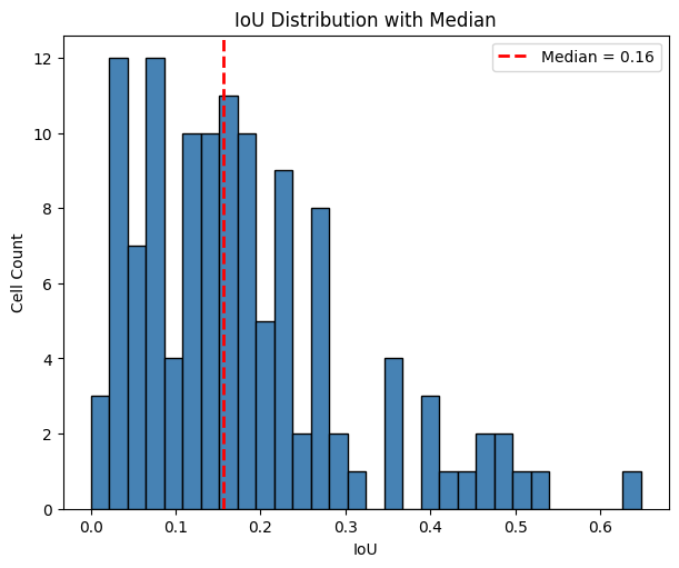
The histogram of IoU distribution (below) shows a median IoU is at 0.16, i.e. 16% overlap.

import matplotlib.pyplot as plt
import numpy as np

# Prepare IoU values
ious = sdata["table"].obs["IoU"].dropna()
median_iou = np.median(ious)

# Set up figure with histogram
fig, ax = plt.subplots(figsize=(6, 5), constrained_layout=True)

# Plot histogram
ax.hist(ious, bins=30, color="steelblue", edgecolor="black")

# Add median line
ax.axvline(
    median_iou,
    color="red",
    linestyle="--",
    linewidth=2,
    label=f"Median = {median_iou:.2f}",
)

# Decorate
ax.set_title("IoU Distribution with Median")
ax.set_xlabel("IoU")
ax.set_ylabel("Cell Count")
ax.legend()

plt.show()

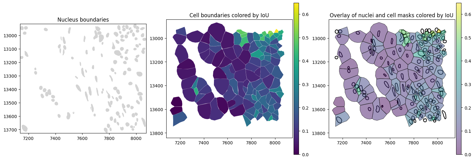
In the spatial plots, we can see that cells that have a high overlap with nuclei, also show a high IoU value.

import matplotlib.pyplot as plt

axes = plt.subplots(1, 3, figsize=(15, 5), constrained_layout=True)[1].flatten()

# link annotations with cell boundaries
sdata.tables["table"].obs["region"] = "cell_boundaries"
sdata.set_table_annotates_spatialelement("table", region="cell_boundaries")

# plot
sdata.pl.render_shapes("nucleus_boundaries").pl.show(
    ax=axes[0], title="Nucleus boundaries", coordinate_systems="global"
)

sdata.pl.render_shapes("cell_boundaries", color="IoU").pl.show(
    ax=axes[1], title="Cell boundaries colored by IoU", coordinate_systems="global"
)

sdata.pl.render_shapes(
    element="nucleus_boundaries",
    fill_alpha=0.2,
    outline_alpha=1.0,
    outline_color="black",
).pl.render_shapes(
    element="cell_boundaries",
    color="IoU",
    cmap="viridis",
    fill_alpha=0.5,
    outline_alpha=1.0,
    outline_width=0.5,
    outline_color="black",
).pl.show(ax=axes[2], title="Overlay of nuclei and cell masks colored by IoU", colorbar=True)

/home/lazic/miniforge3/envs/sc_analysis_sdata/lib/python3.10/site-packages/spatialdata/_core/spatialdata.py:511: UserWarning: Converting `region_key: region` to categorical dtype.
  convert_region_column_to_categorical(table)
/home/lazic/miniforge3/envs/sc_analysis_sdata/lib/python3.10/site-packages/spatialdata/_core/_elements.py:105: UserWarning: Key `cell_boundaries` already exists. Overwriting it in-memory.
  self._check_key(key, self.keys(), self._shared_keys)
/home/lazic/miniforge3/envs/sc_analysis_sdata/lib/python3.10/site-packages/spatialdata/_core/_elements.py:125: UserWarning: Key `table` already exists. Overwriting it in-memory.
  self._check_key(key, self.keys(), self._shared_keys)
/home/lazic/miniforge3/envs/sc_analysis_sdata/lib/python3.10/site-packages/spatialdata/_core/_elements.py:105: UserWarning: Key `cell_boundaries` already exists. Overwriting it in-memory.
  self._check_key(key, self.keys(), self._shared_keys)
/home/lazic/miniforge3/envs/sc_analysis_sdata/lib/python3.10/site-packages/spatialdata/_core/_elements.py:125: UserWarning: Key `table` already exists. Overwriting it in-memory.
  self._check_key(key, self.keys(), self._shared_keys)

Expression correlation between cell and nucleus

Expression correlation between a cell and the “most-overlapping” nucleus can be computed using compute_cell_nuc_correlation. This function will internally compute IoU using compute_cell_nuc_ious unless already present in the spatialdataobject. Currently only pearsoncorrelation is supported. More options will be added later.

import time

import segtraq as st

start = time.time()
corr_df = st.nc.compute_cell_nuc_correlation(sdata)
end = time.time()

print(f"Elapsed time without computing IoU: {end - start:.2f} seconds")

/home/lazic/miniforge3/envs/sc_analysis_sdata/lib/python3.10/site-packages/spatialdata/_core/operations/aggregate.py:452: FutureWarning: The default of observed=False is deprecated and will be changed to True in a future version of pandas. Pass observed=False to retain current behavior or observed=True to adopt the future default and silence this warning.
  aggregated = joined.groupby([INDEX, vk])[ONES_COLUMN].agg(agg_func).reset_index()
/home/lazic/miniforge3/envs/sc_analysis_sdata/lib/python3.10/site-packages/anndata/_core/aligned_df.py:68: ImplicitModificationWarning: Transforming to str index.
  warnings.warn("Transforming to str index.", ImplicitModificationWarning)
/home/lazic/miniforge3/envs/sc_analysis_sdata/lib/python3.10/site-packages/spatialdata/models/models.py:1144: UserWarning: Converting `region_key: region` to categorical dtype.
  return convert_region_column_to_categorical(adata)

Elapsed time without computing IoU: 0.85 seconds

corr_df

	cell_id	best_nuc_id	IoU	correlation
0	4613	4613	0.094093	0.272743
1	4614	4614	0.207238	0.878210
2	4615	4615	0.178686	0.739670
3	4616	4616	0.292909	0.779925
4	4617	4617	0.161824	0.910924
...	...	...	...	...
117	80759	80759	0.160499	0.812877
118	80760	80760	0.128202	0.914975
119	80761	80761	0.288906	0.913159
120	80762	80762	0.180239	0.913756
121	80763	80763	0.269007	0.733573

122 rows × 4 columns

We will store the results in the .obs of the Table within the sdata object for plotting.

corr_df = corr_df.set_index("cell_id")

sdata["table"].obs["pearson_corr"] = sdata["table"].obs["cell_id"].map(corr_df["correlation"])

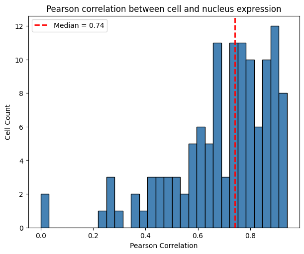
The histogram below shows the distribution of Pearson correlation values across cells. It is right-skewed, with a median of 0.74. This provides intuition about possible spatial spillover: cells may be contaminated by neighboring cells, assuming that nuclei capture expression with less contamination due to their smaller radius.

# Prepare corr values
obs = sdata["table"].obs
corr = obs["pearson_corr"]
median_corr = np.median(corr)

# Set up figure with histogram
fig, ax = plt.subplots(figsize=(6, 5), constrained_layout=True)

# Plot histogram
ax.hist(corr, bins=30, color="steelblue", edgecolor="black")

# Add median line
ax.axvline(
    median_corr,
    color="red",
    linestyle="--",
    linewidth=2,
    label=f"Median = {median_corr:.2f}",
)

# Decorate
ax.set_title("Pearson correlation between cell and nucleus expression")
ax.set_xlabel("Pearson Correlation")
ax.set_ylabel("Cell Count")
ax.legend()

plt.show()

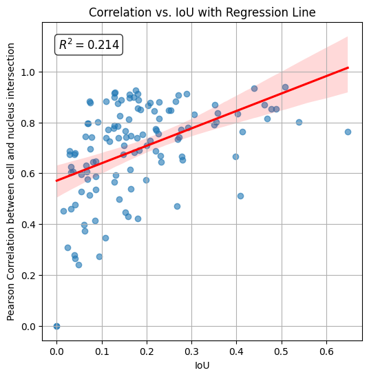
The calculated R2 (coefficient of determination) is 0.214 indicating that correlation between cell and nucleus increases with their IoU.

import seaborn as sns
from scipy.stats import linregress

# Extract the relevant columns, excluding NaNs
df = obs[["IoU", "pearson_corr"]].dropna()

# Compute regression metrics
slope, intercept, r_value, p_value, std_err = linregress(df["IoU"], df["pearson_corr"])
r_squared = r_value**2

# Create the plot
plt.figure(figsize=(6, 6))
ax = sns.regplot(
    data=df,
    x="IoU",
    y="pearson_corr",
    scatter_kws={"alpha": 0.6},
    line_kws={"color": "red"},
    ci=95,
)

# Overlay the R² value
ax.text(
    0.05,
    0.95,
    f"$R^2 = {r_squared:.3f}$",
    transform=ax.transAxes,
    verticalalignment="top",
    fontsize=12,
    bbox=dict(boxstyle="round,pad=0.3", facecolor="white", alpha=0.8),
)

ax.set_xlabel("IoU")
ax.set_ylabel("Pearson Correlation between cell and nucleus intersection")
ax.set_title("Correlation vs. IoU with Regression Line")
ax.grid(True)

plt.show()

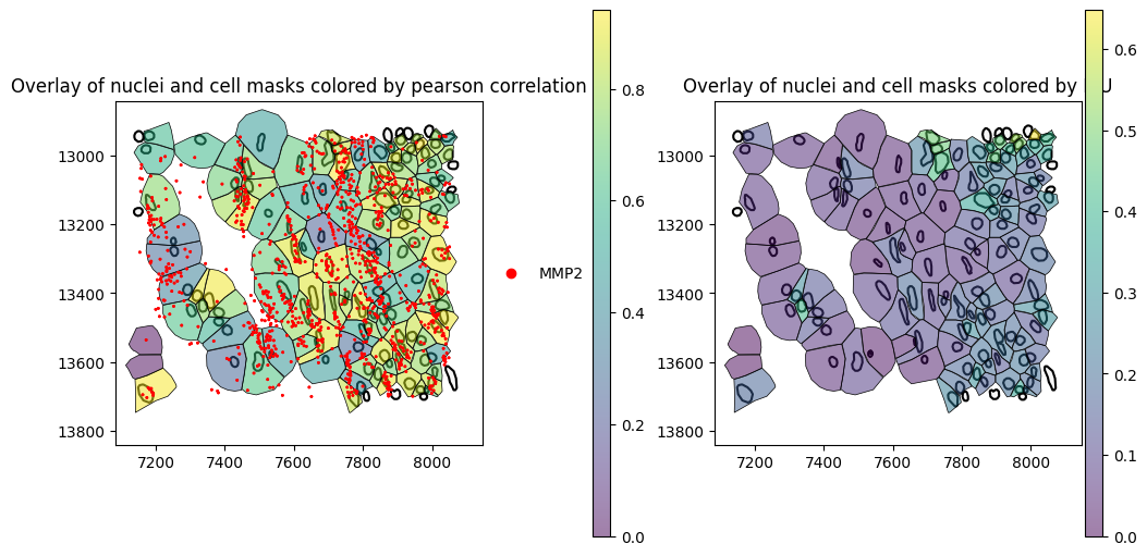
The spatial plot below overlays nucleus boundaries, cell masks colored by Pearson correlation, and transcripts. Cells whose transcripts are distributed across the nucleus region tend to have higher correlation with the nucleus, while cells whose transcripts are localized outside the nuclear region—potentially due to spillover from neighboring cells—tend to exhibit lower correlation.

# link annotations with cell boundaries
sdata.tables["table"].obs["region"] = "cell_boundaries"
sdata.set_table_annotates_spatialelement("table", region="cell_boundaries")

axes = plt.subplots(1, 2, figsize=(10, 5), constrained_layout=True)[1].flatten()

sdata.pl.render_shapes(
    element="nucleus_boundaries",
    fill_alpha=0.2,
    outline_alpha=1.0,
    outline_color="black",
).pl.render_shapes(
    element="cell_boundaries",
    color="pearson_corr",
    cmap="viridis",
    fill_alpha=0.5,
    outline_alpha=1.0,
    outline_width=0.5,
    outline_color="black",
).pl.render_points(
    "transcripts",
    color="feature_name",
    groups="MMP2",
    palette="red",
).pl.show(
    ax=axes[0],
    title="Overlay of nuclei and cell masks colored by pearson correlation",
    colorbar=True,
    figsize=(6, 6),
)


sdata.pl.render_shapes(
    element="nucleus_boundaries",
    fill_alpha=0.2,
    outline_alpha=1.0,
    outline_color="black",
).pl.render_shapes(
    element="cell_boundaries",
    color="IoU",
    cmap="viridis",
    fill_alpha=0.5,
    outline_alpha=1.0,
    outline_width=0.5,
    outline_color="black",
).pl.show(
    ax=axes[1],
    title="Overlay of nuclei and cell masks colored by IoU",
    colorbar=True,
    figsize=(6, 6),
)

/home/lazic/miniforge3/envs/sc_analysis_sdata/lib/python3.10/site-packages/spatialdata/_core/spatialdata.py:511: UserWarning: Converting `region_key: region` to categorical dtype.
  convert_region_column_to_categorical(table)
/home/lazic/miniforge3/envs/sc_analysis_sdata/lib/python3.10/site-packages/spatialdata/_core/_elements.py:105: UserWarning: Key `cell_boundaries` already exists. Overwriting it in-memory.
  self._check_key(key, self.keys(), self._shared_keys)
/home/lazic/miniforge3/envs/sc_analysis_sdata/lib/python3.10/site-packages/spatialdata/_core/_elements.py:125: UserWarning: Key `table` already exists. Overwriting it in-memory.
  self._check_key(key, self.keys(), self._shared_keys)
/home/lazic/miniforge3/envs/sc_analysis_sdata/lib/python3.10/site-packages/anndata/_core/anndata.py:381: FutureWarning: The dtype argument is deprecated and will be removed in late 2024.
  warnings.warn(
/home/lazic/miniforge3/envs/sc_analysis_sdata/lib/python3.10/site-packages/anndata/_core/aligned_df.py:68: ImplicitModificationWarning: Transforming to str index.
  warnings.warn("Transforming to str index.", ImplicitModificationWarning)
/home/lazic/miniforge3/envs/sc_analysis_sdata/lib/python3.10/site-packages/spatialdata/_core/_elements.py:115: UserWarning: Key `transcripts` already exists. Overwriting it in-memory.
  self._check_key(key, self.keys(), self._shared_keys)

INFO     input has more than 103 categories. Uniform 'grey' color will be used for all categories.

/home/lazic/miniforge3/envs/sc_analysis_sdata/lib/python3.10/site-packages/spatialdata_plot/pl/utils.py:775: FutureWarning: The default value of 'ignore' for the `na_action` parameter in pandas.Categorical.map is deprecated and will be changed to 'None' in a future version. Please set na_action to the desired value to avoid seeing this warning
  color_vector = color_source_vector.map(color_mapping)
/home/lazic/miniforge3/envs/sc_analysis_sdata/lib/python3.10/site-packages/spatialdata_plot/pl/render.py:682: UserWarning: No data for colormapping provided via 'c'. Parameters 'cmap', 'norm' will be ignored
  _cax = ax.scatter(
/home/lazic/miniforge3/envs/sc_analysis_sdata/lib/python3.10/site-packages/spatialdata/_core/_elements.py:105: UserWarning: Key `cell_boundaries` already exists. Overwriting it in-memory.
  self._check_key(key, self.keys(), self._shared_keys)
/home/lazic/miniforge3/envs/sc_analysis_sdata/lib/python3.10/site-packages/spatialdata/_core/_elements.py:125: UserWarning: Key `table` already exists. Overwriting it in-memory.
  self._check_key(key, self.keys(), self._shared_keys)

Correlation between Intersection and Remainder Parts of the Cell

The function compute_correlation_between_parts() computes the Pearson correlation between the spatial transcript feature counts within the intersection of a cell and its matched nucleus, and the remainder of the cell. It returns NaN when the regions have no overlapping transcripts or lack sufficient variability. A low correlation may indicate that the cell boundary extension captures neighborhood or ambient signal rather than true intracellular expression—a concern similarly highlighted by segmentation benchmarks such as Baysor. This is based on the assumption that transcripts are homogeneously distributed within the cell and not localized in specific subcellular regions.

start = time.time()
corr_parts_df = st.nc.compute_correlation_between_parts(sdata)
end = time.time()

print(f"Elapsed time without computing IoU: {end - start:.2f} seconds")

Computing correlations: 122it [00:02, 59.79it/s]

Elapsed time without computing IoU: 2.07 seconds

len(corr_parts_df) == len(sdata.tables["table"].obs)

True

We will store the results in the .obs of the Table within the sdata object for plotting.

corr_parts_df = corr_parts_df.set_index("cell_id")

sdata["table"].obs["pearson_corr_parts"] = sdata["table"].obs["cell_id"].map(corr_parts_df["correlation_parts"])

sdata["table"].obs

	cell_id	transcript_counts	control_probe_counts	control_codeword_counts	total_counts	cell_area	nucleus_area	region	IoU	best_nuc_id	pearson_corr	pearson_corr_parts
4612	4613	210	0	0	210	272.066406	27.319531	cell_boundaries	0.094093	4613	0.272743	0.113081
4613	4614	192	0	0	192	154.208594	33.280156	cell_boundaries	0.207238	4614	0.878210	0.529910
4614	4615	174	0	0	174	170.193906	31.744844	cell_boundaries	0.178686	4615	0.739670	0.289943
4615	4616	70	0	0	70	85.796875	26.235781	cell_boundaries	0.292909	4616	0.779925	0.258221
4616	4617	85	0	0	85	101.737031	16.843281	cell_boundaries	0.161824	4617	0.910924	0.761505
...	...	...	...	...	...	...	...	...	...	...	...	...
80758	80759	227	0	0	227	256.984219	42.221094	cell_boundaries	0.160499	80759	0.812877	0.628438
80759	80760	198	0	0	198	222.800938	30.028906	cell_boundaries	0.128202	80760	0.914975	0.896952
80760	80761	110	0	0	110	111.355313	33.144688	cell_boundaries	0.288906	80761	0.913159	0.751234
80761	80762	150	0	0	150	322.189844	60.644844	cell_boundaries	0.180239	80762	0.913756	0.786104
80762	80763	109	0	0	109	152.763594	41.769531	cell_boundaries	0.269007	80763	0.733573	0.360049

122 rows × 12 columns

sdata["table"].obs["pearson_corr_parts"].isna().sum()

np.int64(2)

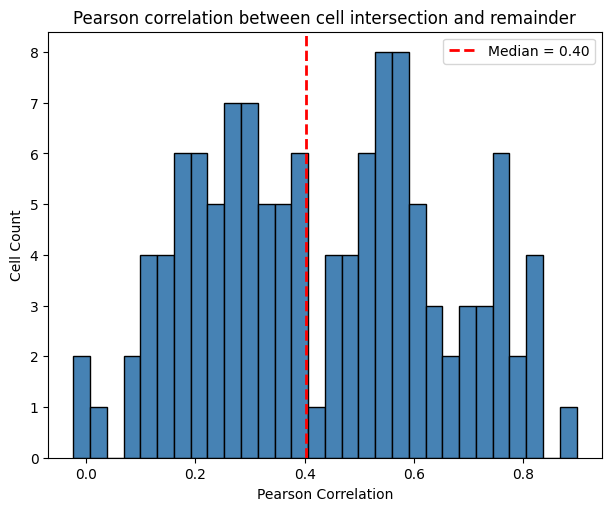
The histogram below shows that the Pearson correlation between the intersection and remainder region of the cell is 0.4.

obs = sdata["table"].obs
# Prepare corr_parts values
corr = obs["pearson_corr_parts"]
median_corr_parts = corr.median()

# Set up figure with histogram
fig, ax = plt.subplots(figsize=(6, 5), constrained_layout=True)

# Plot histogram
ax.hist(corr, bins=30, color="steelblue", edgecolor="black")

# Add median line
ax.axvline(
    median_corr_parts,
    color="red",
    linestyle="--",
    linewidth=2,
    label=f"Median = {median_corr_parts:.2f}",
)

# Decorate
ax.set_title("Pearson correlation between cell intersection and remainder")
ax.set_xlabel("Pearson Correlation")
ax.set_ylabel("Cell Count")
ax.legend()

plt.show()

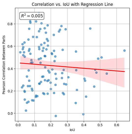
The histogram below visualizes the Pearson correlation between transcript counts in the intersection and remainder of each cell, plotted against the Intersection over Union (IoU) with the nucleus. The calculated R2 (coefficient of determination) value is 0.005, indicating that IoU explains less than 1% of the variance in correlation. This negligible relationship suggests that normalization of the correlation metric by IoU is not necessary.

import seaborn as sns

# Extract the relevant columns, excluding NaNs
df = obs[["IoU", "pearson_corr_parts"]].dropna()

# Compute regression metrics
slope, intercept, r_value, p_value, std_err = linregress(df["IoU"], df["pearson_corr_parts"])
r_squared = r_value**2

# Create the plot
plt.figure(figsize=(6, 6))
ax = sns.regplot(
    data=df,
    x="IoU",
    y="pearson_corr_parts",
    scatter_kws={"alpha": 0.6},
    line_kws={"color": "red"},
    ci=95,
)

# Overlay the R² value
ax.text(
    0.05,
    0.95,
    f"$R^2 = {r_squared:.3f}$",
    transform=ax.transAxes,
    verticalalignment="top",
    fontsize=12,
    bbox=dict(boxstyle="round,pad=0.3", facecolor="white", alpha=0.8),
)

ax.set_xlabel("IoU")
ax.set_ylabel("Pearson Correlation Between Parts")
ax.set_title("Correlation vs. IoU with Regression Line")
ax.grid(True)

plt.show()

Because spatialdata-plot plots all boundaries in grey, if there are NaN values in the annotation (describe before), we will copy the pearson_corr_parts column and set NaNvalues to 0.0just for plotting. We will try to solve this issue later.

sdata["table"].obs["pearson_corr_parts_plot"] = (
    sdata["table"].obs["cell_id"].map(corr_parts_df["correlation_parts"])
)  # TODO
sdata["table"].obs.loc[sdata["table"].obs["pearson_corr_parts_plot"].isna(), "pearson_corr_parts_plot"] = 0.0

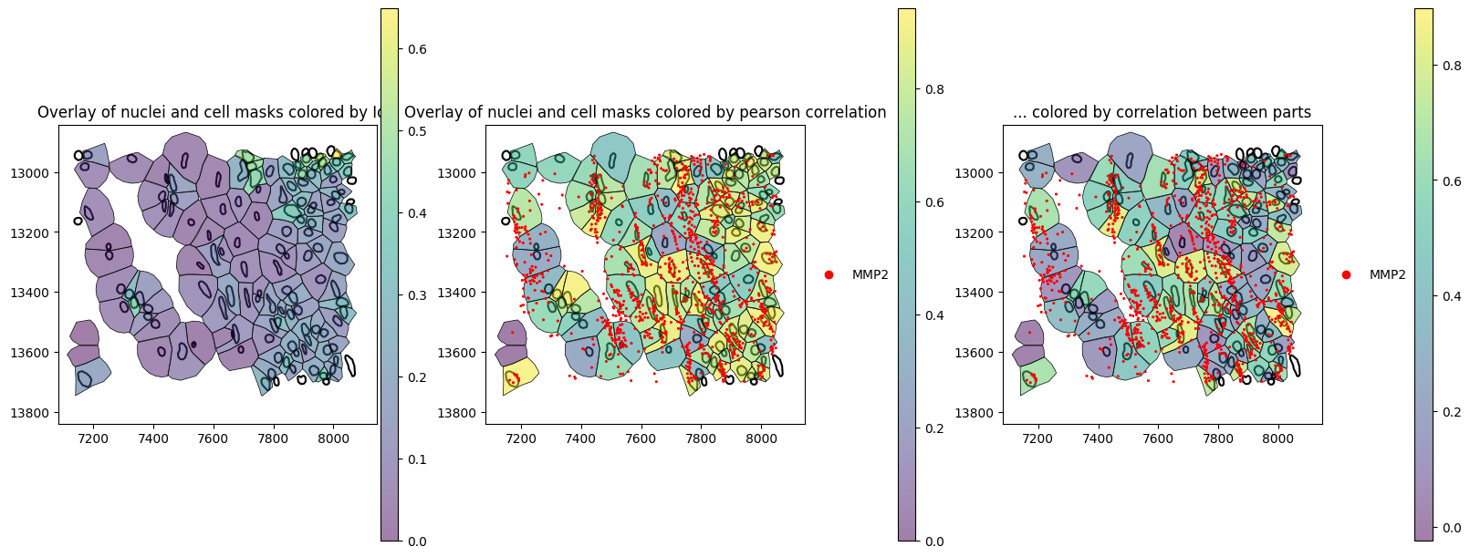
The spatial plots below shows the spatial distribution of computed correlations. The Pearson correlation between parts can be a measure of how much neighboring signal is captured.

# link annotations with cell boundaries
sdata.tables["table"].obs["region"] = "cell_boundaries"
sdata.set_table_annotates_spatialelement("table", region="cell_boundaries")

axes = plt.subplots(1, 3, figsize=(16, 6), constrained_layout=True)[1].flatten()

sdata.pl.render_shapes(
    element="nucleus_boundaries",
    fill_alpha=0.2,
    outline_alpha=1.0,
    outline_color="black",
).pl.render_shapes(
    element="cell_boundaries",
    color="IoU",
    cmap="viridis",
    fill_alpha=0.5,
    outline_alpha=1.0,
    outline_width=0.5,
    outline_color="black",
).pl.show(
    ax=axes[0],
    title="Overlay of nuclei and cell masks colored by IoU",
    colorbar=True,
    figsize=(6, 6),
)

sdata.pl.render_shapes(
    element="nucleus_boundaries",
    fill_alpha=0.2,
    outline_alpha=1.0,
    outline_color="black",
).pl.render_shapes(
    element="cell_boundaries",
    color="pearson_corr",
    cmap="viridis",
    fill_alpha=0.5,
    outline_alpha=1.0,
    outline_width=0.5,
    outline_color="black",
).pl.render_points(
    "transcripts",
    color="feature_name",
    groups="MMP2",
    palette="red",
).pl.show(
    ax=axes[1],
    title="Overlay of nuclei and cell masks colored by pearson correlation",
    colorbar=True,
    figsize=(6, 6),
)

sdata.pl.render_shapes(
    element="nucleus_boundaries",
    fill_alpha=0.2,
    outline_alpha=1.0,
    outline_color="black",
).pl.render_shapes(
    element="cell_boundaries",
    color="pearson_corr_parts_plot",
    cmap="viridis",
    fill_alpha=0.5,
    outline_alpha=1.0,
    outline_width=0.5,
    outline_color="black",
).pl.render_points(
    "transcripts",
    color="feature_name",
    groups="MMP2",
    palette="red",
).pl.show(
    ax=axes[2],
    title="... colored by correlation between parts",
    colorbar=True,
    figsize=(6, 6),
)

# remove column again
sdata["table"].obs.drop(columns=["pearson_corr_parts_plot"], inplace=True)

/home/lazic/miniforge3/envs/sc_analysis_sdata/lib/python3.10/site-packages/spatialdata/_core/spatialdata.py:511: UserWarning: Converting `region_key: region` to categorical dtype.
  convert_region_column_to_categorical(table)
/home/lazic/miniforge3/envs/sc_analysis_sdata/lib/python3.10/site-packages/spatialdata/_core/_elements.py:105: UserWarning: Key `cell_boundaries` already exists. Overwriting it in-memory.
  self._check_key(key, self.keys(), self._shared_keys)
/home/lazic/miniforge3/envs/sc_analysis_sdata/lib/python3.10/site-packages/spatialdata/_core/_elements.py:125: UserWarning: Key `table` already exists. Overwriting it in-memory.
  self._check_key(key, self.keys(), self._shared_keys)

INFO     input has more than 103 categories. Uniform 'grey' color will be used for all categories.

/home/lazic/miniforge3/envs/sc_analysis_sdata/lib/python3.10/site-packages/spatialdata/_core/_elements.py:105: UserWarning: Key `cell_boundaries` already exists. Overwriting it in-memory.
  self._check_key(key, self.keys(), self._shared_keys)
/home/lazic/miniforge3/envs/sc_analysis_sdata/lib/python3.10/site-packages/spatialdata/_core/_elements.py:125: UserWarning: Key `table` already exists. Overwriting it in-memory.
  self._check_key(key, self.keys(), self._shared_keys)
/home/lazic/miniforge3/envs/sc_analysis_sdata/lib/python3.10/site-packages/anndata/_core/anndata.py:381: FutureWarning: The dtype argument is deprecated and will be removed in late 2024.
  warnings.warn(
/home/lazic/miniforge3/envs/sc_analysis_sdata/lib/python3.10/site-packages/anndata/_core/aligned_df.py:68: ImplicitModificationWarning: Transforming to str index.
  warnings.warn("Transforming to str index.", ImplicitModificationWarning)
/home/lazic/miniforge3/envs/sc_analysis_sdata/lib/python3.10/site-packages/spatialdata/_core/_elements.py:115: UserWarning: Key `transcripts` already exists. Overwriting it in-memory.
  self._check_key(key, self.keys(), self._shared_keys)
/home/lazic/miniforge3/envs/sc_analysis_sdata/lib/python3.10/site-packages/spatialdata_plot/pl/utils.py:775: FutureWarning: The default value of 'ignore' for the `na_action` parameter in pandas.Categorical.map is deprecated and will be changed to 'None' in a future version. Please set na_action to the desired value to avoid seeing this warning
  color_vector = color_source_vector.map(color_mapping)
/home/lazic/miniforge3/envs/sc_analysis_sdata/lib/python3.10/site-packages/spatialdata_plot/pl/render.py:682: UserWarning: No data for colormapping provided via 'c'. Parameters 'cmap', 'norm' will be ignored
  _cax = ax.scatter(

INFO     input has more than 103 categories. Uniform 'grey' color will be used for all categories.

/home/lazic/miniforge3/envs/sc_analysis_sdata/lib/python3.10/site-packages/spatialdata/_core/_elements.py:105: UserWarning: Key `cell_boundaries` already exists. Overwriting it in-memory.
  self._check_key(key, self.keys(), self._shared_keys)
/home/lazic/miniforge3/envs/sc_analysis_sdata/lib/python3.10/site-packages/spatialdata/_core/_elements.py:125: UserWarning: Key `table` already exists. Overwriting it in-memory.
  self._check_key(key, self.keys(), self._shared_keys)
/home/lazic/miniforge3/envs/sc_analysis_sdata/lib/python3.10/site-packages/anndata/_core/anndata.py:381: FutureWarning: The dtype argument is deprecated and will be removed in late 2024.
  warnings.warn(
/home/lazic/miniforge3/envs/sc_analysis_sdata/lib/python3.10/site-packages/anndata/_core/aligned_df.py:68: ImplicitModificationWarning: Transforming to str index.
  warnings.warn("Transforming to str index.", ImplicitModificationWarning)
/home/lazic/miniforge3/envs/sc_analysis_sdata/lib/python3.10/site-packages/spatialdata/_core/_elements.py:115: UserWarning: Key `transcripts` already exists. Overwriting it in-memory.
  self._check_key(key, self.keys(), self._shared_keys)
/home/lazic/miniforge3/envs/sc_analysis_sdata/lib/python3.10/site-packages/spatialdata_plot/pl/utils.py:775: FutureWarning: The default value of 'ignore' for the `na_action` parameter in pandas.Categorical.map is deprecated and will be changed to 'None' in a future version. Please set na_action to the desired value to avoid seeing this warning
  color_vector = color_source_vector.map(color_mapping)
/home/lazic/miniforge3/envs/sc_analysis_sdata/lib/python3.10/site-packages/spatialdata_plot/pl/render.py:682: UserWarning: No data for colormapping provided via 'c'. Parameters 'cmap', 'norm' will be ignored
  _cax = ax.scatter(