Label transfer from scRNA-seq dataset via Pearson correlation#
In this notebook, we will show how to transfer labels from a reference single-cell RNA-sequencing (scRNA-seq) dataset via a lightweight approach. We will use Pearson correlation to find the celltype with the highest expression correlation for each cell the spatial transcriptomics datasset, according to CellSPA.
Load scRNA-seq dataset#
We use the scRNA-seq dataset of diffuse large B-cell lymphoma (DLBCL) samples from Dong et al. published on CellxGene.
[1]:
from pathlib import Path

import anndata as ad

scRNAseq_data_path = Path("/g/huber/projects/CODEX/segtraq/data/label_transfer/scRNA_seq_DLBCL_matched_with_2_C1.h5ad")
adata_ref = ad.read(scRNAseq_data_path)
/home/lazic/miniforge3/envs/sc_analysis_sdata/lib/python3.10/site-packages/anndata/__init__.py:42: FutureWarning: `anndata.read` is deprecated, use `anndata.read_h5ad` instead. `ad.read` will be removed in mid 2024.
  warnings.warn(
[2]:
adata_ref
[2]:
AnnData object with n_obs × n_vars = 29184 × 442
    obs: 'cell_type', 'is_primary_data', 'sample_id'
The counts in the reference dataset are already log-normalized, so we can copy that matrix to a layer called ‘logcounts’.
[3]:
adata_ref.X.toarray()
[3]:
array([[0.        , 0.        , 0.        , ..., 0.        , 0.        ,
        0.        ],
       [0.        , 0.        , 0.        , ..., 0.        , 0.        ,
        0.        ],
       [0.        , 0.        , 2.38975334, ..., 0.        , 0.        ,
        0.        ],
       ...,
       [0.        , 0.        , 0.        , ..., 0.        , 0.        ,
        0.        ],
       [0.        , 0.        , 0.        , ..., 0.        , 0.        ,
        0.        ],
       [0.        , 0.        , 0.        , ..., 0.        , 0.        ,
        0.        ]], shape=(29184, 442))
[4]:
adata_ref.layers["logcounts"] = adata_ref.X.copy()
We aggregate log-normalized gene expression values (logcounts) across cells grouped by their annotated cell type, computing the mean expression per gene within each cell type. This yields a reference expression profile for each cell type.
[5]:
import numpy as np

logcounts = adata_ref.layers["logcounts"]
# If it's sparse, convert to dense
if not isinstance(logcounts, np.ndarray):
    logcounts = logcounts.toarray()

celltypes = adata_ref.obs["cell_type"]
[6]:
import pandas as pd

logcounts_df = pd.DataFrame(logcounts, columns=adata_ref.var_names)
logcounts_df["celltype"] = celltypes.values

ref_mean_df = logcounts_df.groupby("celltype").mean()
/tmp/ipykernel_3092810/2272690639.py:6: FutureWarning: The default of observed=False is deprecated and will be changed to True in a future version of pandas. Pass observed=False to retain current behavior or observed=True to adopt the future default and silence this warning.
  ref_mean_df = logcounts_df.groupby("celltype").mean()
[7]:
ref_mean_df
[7]:
| A2M | ABCA1 | ACACA | ACADM | ACKR1 | ACKR4 | ACTA2 | ADAM10 | ADAM17 | ADCY7 | ... | IL9 | IGLC3 | HMGB1 | GNAS | IL22 | IGLC2 | DRAIC | ANGPT2 | ICOSLG | IL6ST | |
|---|---|---|---|---|---|---|---|---|---|---|---|---|---|---|---|---|---|---|---|---|---|
| celltype | |||||||||||||||||||||
| B | 0.000000 | 0.016769 | 0.156024 | 0.159486 | 0.000000 | 0.022256 | 0.050791 | 0.213838 | 0.229673 | 0.270148 | ... | 0.0 | 0.0 | 0.0 | 0.0 | 0.0 | 0.0 | 0.0 | 0.0 | 0.0 | 0.0 |
| DC_pc | 0.036694 | 0.169812 | 0.117063 | 0.444065 | 0.004440 | 0.003707 | 0.140305 | 0.437622 | 0.294588 | 0.784672 | ... | 0.0 | 0.0 | 0.0 | 0.0 | 0.0 | 0.0 | 0.0 | 0.0 | 0.0 | 0.0 |
| Endothelia | 1.471162 | 0.178528 | 0.270104 | 0.289596 | 0.885165 | 0.013624 | 0.112109 | 0.361705 | 0.256111 | 0.163421 | ... | 0.0 | 0.0 | 0.0 | 0.0 | 0.0 | 0.0 | 0.0 | 0.0 | 0.0 | 0.0 |
| Epithelia | 0.019746 | 0.080427 | 0.254660 | 0.178775 | 0.001124 | 0.026345 | 0.017461 | 0.119152 | 0.206132 | 0.108029 | ... | 0.0 | 0.0 | 0.0 | 0.0 | 0.0 | 0.0 | 0.0 | 0.0 | 0.0 | 0.0 |
| Fibro_Muscle | 0.266040 | 0.312430 | 0.264807 | 0.343359 | 0.072844 | 0.003145 | 0.434594 | 0.369848 | 0.277516 | 0.193193 | ... | 0.0 | 0.0 | 0.0 | 0.0 | 0.0 | 0.0 | 0.0 | 0.0 | 0.0 | 0.0 |
| Mono_Macro | 0.656003 | 0.890168 | 0.149249 | 0.331428 | 0.014655 | 0.002430 | 0.114052 | 0.358778 | 0.334295 | 0.585345 | ... | 0.0 | 0.0 | 0.0 | 0.0 | 0.0 | 0.0 | 0.0 | 0.0 | 0.0 | 0.0 |
| NK | 0.021211 | 0.106054 | 0.201798 | 0.357114 | 0.005284 | 0.000000 | 0.101637 | 0.559331 | 0.245895 | 0.659352 | ... | 0.0 | 0.0 | 0.0 | 0.0 | 0.0 | 0.0 | 0.0 | 0.0 | 0.0 | 0.0 |
| Pericyte | 2.253352 | 0.360183 | 0.252609 | 0.435539 | 0.326374 | 0.000000 | 0.803320 | 0.553716 | 0.318709 | 0.157481 | ... | 0.0 | 0.0 | 0.0 | 0.0 | 0.0 | 0.0 | 0.0 | 0.0 | 0.0 | 0.0 |
| T_CD4 | 0.029272 | 0.077661 | 0.152805 | 0.257307 | 0.008759 | 0.000000 | 0.137884 | 0.459278 | 0.233179 | 0.363228 | ... | 0.0 | 0.0 | 0.0 | 0.0 | 0.0 | 0.0 | 0.0 | 0.0 | 0.0 | 0.0 |
| T_CD8 | 0.031461 | 0.045086 | 0.151711 | 0.311616 | 0.004273 | 0.001105 | 0.106523 | 0.336085 | 0.214291 | 0.386563 | ... | 0.0 | 0.0 | 0.0 | 0.0 | 0.0 | 0.0 | 0.0 | 0.0 | 0.0 | 0.0 |
| T_dividing | 0.051053 | 0.032399 | 0.196901 | 0.487031 | 0.003520 | 0.000000 | 0.150578 | 0.765854 | 0.408252 | 0.345907 | ... | 0.0 | 0.0 | 0.0 | 0.0 | 0.0 | 0.0 | 0.0 | 0.0 | 0.0 | 0.0 |
| Tumor_DLBCL | 0.017330 | 0.074456 | 0.278579 | 0.419433 | 0.004762 | 0.000889 | 0.196989 | 0.418151 | 0.366993 | 0.365700 | ... | 0.0 | 0.0 | 0.0 | 0.0 | 0.0 | 0.0 | 0.0 | 0.0 | 0.0 | 0.0 |
| cDC | 0.077264 | 0.341498 | 0.163797 | 0.296956 | 0.021874 | 0.005103 | 0.095915 | 0.394451 | 0.305254 | 0.900343 | ... | 0.0 | 0.0 | 0.0 | 0.0 | 0.0 | 0.0 | 0.0 | 0.0 | 0.0 | 0.0 |
13 rows × 442 columns
Load spatialData object#
Next, we load the spatialdata object of a Xenium DLBCL sample.
[8]:
import spatialdata as sd

sdata = sd.read_zarr(
    "/g/huber/projects/GSK_lazic/B_NHL/BNHL_RICOVER/tma_2/2_C1/proseg_output/spatialData_2_C1_proseg.zarr"
)
/home/lazic/miniforge3/envs/sc_analysis_sdata/lib/python3.10/site-packages/dask/dataframe/__init__.py:31: FutureWarning: The legacy Dask DataFrame implementation is deprecated and will be removed in a future version. Set the configuration option `dataframe.query-planning` to `True` or None to enable the new Dask Dataframe implementation and silence this warning.
  warnings.warn(
/home/lazic/miniforge3/envs/sc_analysis_sdata/lib/python3.10/site-packages/xarray_schema/__init__.py:1: UserWarning: pkg_resources is deprecated as an API. See https://setuptools.pypa.io/en/latest/pkg_resources.html. The pkg_resources package is slated for removal as early as 2025-11-30. Refrain from using this package or pin to Setuptools<81.
  from pkg_resources import DistributionNotFound, get_distribution
version mismatch: detected: RasterFormatV02, requested: FormatV04
/home/lazic/miniforge3/envs/sc_analysis_sdata/lib/python3.10/site-packages/zarr/creation.py:614: UserWarning: ignoring keyword argument 'read_only'
  compressor, fill_value = _kwargs_compat(compressor, fill_value, kwargs)
We perform quality control steps (filtering based on #transcripts and #genes per cell) and log-normalization.
[9]:
adata = sdata["table"]
[131]:
import scanpy as sc

import segtraq as st

# Compute QC metrics
transcript_counts = st.bl.transcripts_per_cell(sdata)
gene_counts = st.bl.genes_per_cell(sdata)

transcript_counts.index = transcript_counts.index.astype(str)
gene_counts.index = gene_counts.index.astype(str)

transcript_counts_filtered = transcript_counts.loc[adata.obs_names]
gene_counts_filtered = gene_counts.loc[adata.obs_names]

adata.obs["total_transcripts"] = transcript_counts_filtered["transcript_count"]
adata.obs["total_genes"] = gene_counts_filtered["gene_count"]
[144]:
adata.obs
[144]:
| centroid_x | centroid_y | cell_size | axis_minor_length | axis_major_length | centroid-0 | centroid-1 | eccentricity | solidity | perimeter | sample_id | TMA | region | mask_id | total_transcripts | total_genes | |
|---|---|---|---|---|---|---|---|---|---|---|---|---|---|---|---|---|
| cell_id | ||||||||||||||||
| 1 | 377.79850 | 513.17664 | 395.71875 | 6.590376 | 8.878127 | 512.720930 | 376.953488 | 0.670050 | 0.860000 | 24.899495 | 2_C1 | 2 | cell_labels | 1 | 993 | 73 |
| 2 | 349.86170 | 643.56384 | 92.53125 | 2.653300 | 5.366563 | 643.600000 | 349.000000 | 0.869227 | 0.500000 | 0.000000 | 2_C1 | 2 | cell_labels | 2 | 985 | 89 |
| 3 | 401.73760 | 398.32178 | 397.68750 | 5.502993 | 9.527791 | 396.305556 | 400.916667 | 0.816339 | 0.800000 | 21.071068 | 2_C1 | 2 | cell_labels | 3 | 959 | 136 |
| 4 | 257.44656 | 319.80533 | 773.71875 | 9.718573 | 11.625859 | 319.301205 | 257.168675 | 0.548814 | 0.813725 | 34.384776 | 2_C1 | 2 | cell_labels | 4 | 932 | 161 |
| 5 | 195.35858 | 549.35860 | 194.90625 | 3.843169 | 5.055352 | 548.785714 | 194.928571 | 0.649668 | 0.875000 | 11.414214 | 2_C1 | 2 | cell_labels | 5 | 926 | 47 |
| ... | ... | ... | ... | ... | ... | ... | ... | ... | ... | ... | ... | ... | ... | ... | ... | ... |
| 5843 | 539.39000 | 343.35000 | 196.87500 | 6.445665 | 16.611864 | 343.063492 | 539.158730 | 0.921653 | 0.684783 | 40.798990 | 2_C1 | 2 | cell_labels | 5843 | 61 | 85 |
| 5844 | 256.99690 | 636.03420 | 316.96875 | 7.896618 | 12.941854 | 636.506667 | 256.333333 | 0.792277 | 0.842697 | 35.142136 | 2_C1 | 2 | cell_labels | 5844 | 61 | 41 |
| 5845 | 310.64035 | 493.85090 | 112.21875 | 6.976622 | 7.382183 | 493.272727 | 310.151515 | 0.326891 | 0.733333 | 24.727922 | 2_C1 | 2 | cell_labels | 5845 | 60 | 109 |
| 5846 | 366.64166 | 153.53334 | 236.25000 | 8.121170 | 12.488528 | 152.528571 | 366.328571 | 0.759686 | 0.777778 | 36.556349 | 2_C1 | 2 | cell_labels | 5846 | 60 | 46 |
| 5847 | 494.74417 | 190.87209 | 169.31250 | 8.103957 | 8.811781 | 190.180000 | 494.300000 | 0.392685 | 0.847458 | 26.384776 | 2_C1 | 2 | cell_labels | 5847 | 60 | 33 |
5845 rows × 16 columns
[133]:
# Filter outliers
qc_range = {"total_transcripts": (10, 2000), "total_genes": (5, np.inf)}

for key, (low, high) in qc_range.items():
    mask = (adata.obs[key] >= low) & (adata.obs[key] <= high)
    adata = adata[mask.to_numpy()].copy()
[134]:
# Normalize and log-transform
sc.pp.normalize_total(adata, target_sum=1e4)
sc.pp.log1p(adata)
adata.layers["logcounts"] = adata.X.copy()
/home/lazic/miniforge3/envs/sc_analysis_sdata/lib/python3.10/site-packages/legacy_api_wrap/__init__.py:82: UserWarning: Some cells have zero counts
  return fn(*args_all, **kw)
Label transfer via correlation#
Now, we compute the Pearson correlation between each query cell in the processed AnnData object and the mean expression profiles of reference cell types.
We first identify the common genes between the query data and the reference matrix, and then compute a correlation matrix where each entry reflects the similarity between a query cell and a reference cell type.
For each query cell, we:
Assign the most correlated reference cell type (i.e., the one with the highest Pearson correlation),
Store both the correlation value and the predicted cell type.
This provides a label transfer from the reference to the query dataset based on global transcriptomic similarity.
[ ]:
from anndata import AnnData
from scipy.spatial.distance import cdist


def assign_celltype_by_pearson(adata: AnnData, ref_mean_df: pd.DataFrame, layer: str = "logcounts") -> pd.DataFrame:
    """
    Assigns cell types to cells in `adata` by computing Pearson correlation
    with reference expression profiles.

    Parameters
    ----------
    adata : AnnData
        Query dataset with gene expression data in the specified layer.
    ref_mean_df : pd.DataFrame
        Reference expression matrix with shape (cell_types x genes).
    layer : str, default="logcounts"
        Layer in `adata` to use for expression values.

    Returns
    -------
    pd.DataFrame
        DataFrame with `cell_id` and assigned `celltype`.
    """
    # TODO - check if cdist does really Pearson correlation

    # Extract query expression data
    X_query = pd.DataFrame(
        (adata.layers[layer].toarray() if hasattr(adata.layers[layer], "toarray") else adata.layers[layer]),
        index=adata.obs_names,
        columns=adata.var_names,
    )

    # Align gene order
    common_genes = X_query.columns.intersection(ref_mean_df.columns)
    if len(common_genes) == 0:
        raise ValueError("No common genes found between query and reference.")

    X_query = X_query[common_genes]
    X_ref = ref_mean_df[common_genes]

    # Compute Pearson correlation (1 - correlation distance)
    cor_mat = 1 - cdist(X_query.values, X_ref.values, metric="correlation")
    cor_mat_df = pd.DataFrame(cor_mat, index=adata.obs_names, columns=X_ref.index)

    # Assign best-matching reference cell type
    best_celltype = cor_mat_df.idxmax(axis=1)

    # Return as DataFrame
    return pd.DataFrame({"cell_id": adata.obs_names, "celltype": best_celltype.values})
[146]:
result_df = assign_celltype_by_pearson(adata, ref_mean_df)
/tmp/ipykernel_2382657/4082630372.py:48: FutureWarning: The behavior of DataFrame.idxmax with all-NA values, or any-NA and skipna=False, is deprecated. In a future version this will raise ValueError
  best_celltype = cor_mat_df.idxmax(axis=1)
[158]:
result_df["celltype"].value_counts()
[158]:
celltype
Tumor_DLBCL     2293
T_CD8            952
Mono_Macro       789
T_CD4            599
T_dividing       521
Fibro_Muscle     204
cDC              134
Pericyte         123
B                100
Endothelia        62
NK                35
DC_pc             23
Epithelia          6
Name: count, dtype: int64
[156]:
result_df.set_index("cell_id", inplace=True)
adata.obs["celltype_corr"] = result_df.loc[adata.obs_names, "celltype"]
[163]:
# define colors for cell types

col_celltype = {
    "B": "#fb8072",
    "cDC": "#bc80bd",
    "DC_pc": "#910290",
    "Endothelia": "#fdb462",
    "Epithelia": "#959059",
    "Fibro_Muscle": "#fed9a6",
    "Mono_Macro": "#a6cee3",
    "NK": "#2782bb",
    "Pericyte": "#d2cd7e",
    "T_CD4": "#3c7761",
    "T_CD4_reg": "#66a61e",
    "T_CD8": "#66c2a5",
    "T_dividing": "#1b9e77",
    "Tumor_DLBCL": "#d45943",
}
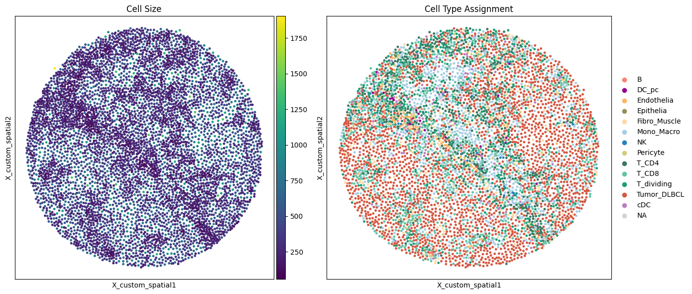
[170]:
import matplotlib.pyplot as plt

# Set up side-by-side plots
fig, axs = plt.subplots(1, 2, figsize=(14, 6))

# Plot 1: Cell size
sc.pl.embedding(
    adata,
    basis="X_custom_spatial",
    color="cell_size",
    size=50,
    ax=axs[0],
    show=False,
    title="Cell Size",
)

# Plot 2: Cell types with custom colors
sc.pl.embedding(
    adata,
    basis="X_custom_spatial",
    color="celltype_corr",
    size=50,
    palette=col_celltype,  # your custom palette from before
    ax=axs[1],
    show=False,
    title="Cell Type Assignment",
)

plt.tight_layout()
plt.show()