Correlations between the top and bottom of the slice

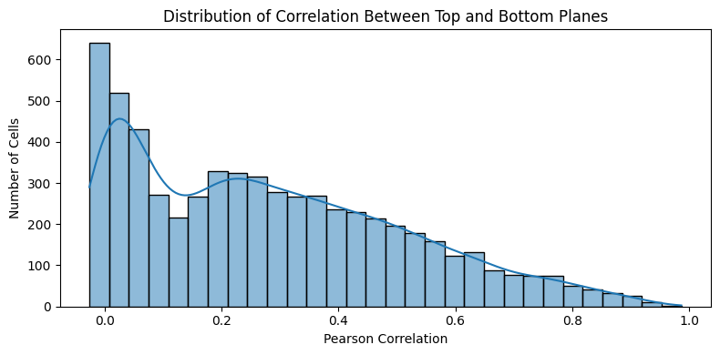
To assess if there are cells lying on top of each other in the z plane, we can slice our data into a top and bottom plane, e. g. by taking the top 25% and the bottom 25%. We can then compute the Pearson correlation between the two planes for each cell. If the correlation is high, the top and bottom layers likely show the same cell. If it is low, there might be two or more cells overlapping in the z direction.

%load_ext autoreload
%autoreload 2

import matplotlib.pyplot as plt
import seaborn as sns
import spatialdata as sd
import squidpy as sq

import segtraq as st

sdata = sd.read_zarr("/g/huber/projects/CODEX/segtraq/data/seg_comparison/spatialData_2_C1_proseg.zarr")

The autoreload extension is already loaded. To reload it, use:
  %reload_ext autoreload

/home/meyerben/meyerben/notebooks/spatial_transcriptomics/SegTraQ/.venv/lib/python3.13/site-packages/anndata/utils.py:434: FutureWarning: Importing read_text from `anndata` is deprecated. Import anndata.io.read_text instead.
  warnings.warn(msg, FutureWarning)
version mismatch: detected: RasterFormatV02, requested: FormatV04
/home/meyerben/meyerben/notebooks/spatial_transcriptomics/SegTraQ/.venv/lib/python3.13/site-packages/zarr/creation.py:610: UserWarning: ignoring keyword argument 'read_only'
  compressor, fill_value = _kwargs_compat(compressor, fill_value, kwargs)

correlation_df = st.cs.compute_z_plane_correlation(sdata)
correlation_df.head()

<string>:35: FutureWarning: The default of observed=False is deprecated and will be changed to True in a future version of pandas. Pass observed=False to retain current behavior or observed=True to adopt the future default and silence this warning.
<string>:36: FutureWarning: The default of observed=False is deprecated and will be changed to True in a future version of pandas. Pass observed=False to retain current behavior or observed=True to adopt the future default and silence this warning.

	correlation
cell_id
UNASSIGNED	0.986754
affmepaj-1	0.668409
affmgdje-1	0.313853
affmgmio-1	0.422878
affmkcka-1	0.570178

# Plot the distribution of correlation values
plt.figure(figsize=(8, 4))
sns.histplot(correlation_df["correlation"], bins=30, kde=True)

plt.title("Distribution of Correlation Between Top and Bottom Planes")
plt.xlabel("Pearson Correlation")
plt.ylabel("Number of Cells")
plt.tight_layout()
plt.show()

# TODO: at this point, we should merge them to the adata object
# unfortunately, the adata object does not contain matching cell IDs, so we cannot do this yet

adata = sdata.tables["table"]

# we need to add the spatial coordinates to the adata object for plotting
adata.obsm["spatial"] = adata.obs[["centroid-0", "centroid-1"]].to_numpy()

# adding the correlation values to the adata object
adata.obs["z_plane_correlation"] = adata.obs.index.map(correlation_df["correlation"])

adata.obs

	centroid_x	centroid_y	cell_size	axis_minor_length	axis_major_length	centroid-0	centroid-1	eccentricity	solidity	perimeter	sample_id	TMA	region	mask_id	z_plane_correlation
cell_id
1	377.79850	513.17664	395.71875	6.590376	8.878127	512.720930	376.953488	0.670050	0.860000	24.899495	2_C1	2	cell_labels	1	NaN
2	349.86170	643.56384	92.53125	2.653300	5.366563	643.600000	349.000000	0.869227	0.500000	0.000000	2_C1	2	cell_labels	2	NaN
3	401.73760	398.32178	397.68750	5.502993	9.527791	396.305556	400.916667	0.816339	0.800000	21.071068	2_C1	2	cell_labels	3	NaN
4	257.44656	319.80533	773.71875	9.718573	11.625859	319.301205	257.168675	0.548814	0.813725	34.384776	2_C1	2	cell_labels	4	NaN
5	195.35858	549.35860	194.90625	3.843169	5.055352	548.785714	194.928571	0.649668	0.875000	11.414214	2_C1	2	cell_labels	5	NaN
...	...	...	...	...	...	...	...	...	...	...	...	...	...	...	...
5843	539.39000	343.35000	196.87500	6.445665	16.611864	343.063492	539.158730	0.921653	0.684783	40.798990	2_C1	2	cell_labels	5843	NaN
5844	256.99690	636.03420	316.96875	7.896618	12.941854	636.506667	256.333333	0.792277	0.842697	35.142136	2_C1	2	cell_labels	5844	NaN
5845	310.64035	493.85090	112.21875	6.976622	7.382183	493.272727	310.151515	0.326891	0.733333	24.727922	2_C1	2	cell_labels	5845	NaN
5846	366.64166	153.53334	236.25000	8.121170	12.488528	152.528571	366.328571	0.759686	0.777778	36.556349	2_C1	2	cell_labels	5846	NaN
5847	494.74417	190.87209	169.31250	8.103957	8.811781	190.180000	494.300000	0.392685	0.847458	26.384776	2_C1	2	cell_labels	5847	NaN

5847 rows × 15 columns

sq.pl.spatial_scatter(
    adata,
    library_id="spatial",
    shape=None,
    color=["z_plane_correlation"],
)