Technology Focus: 10x Genomics Xenium (Simplified)

This tutorial highlights the basic functions of SegTraQ on a single Xenium dataset that was segmented using the Xenium default segmentation. To follow along, you can download the data already in SpatialData format from here.

For a more detailed description of how the data was obtained and a comparison between segmentation methods, please look at the Xenium Focus.

Read SpatialData object

%load_ext autoreload
%autoreload 2

import warnings

import anndata as ad
import dask
import matplotlib.pyplot as plt
import pandas as pd
import scanpy as sc
import seaborn as sns
import spatialdata as sd
import spatialdata_plot  # noqa

import segtraq

segtraq.settings.n_jobs = -1  # Use all available CPU cores

# filtering import and deprecation warnings from spatialdata
# this is in general not recommended
# we only do it here because we have verified that the warnings are irrelevant in this notebook
warnings.simplefilter("ignore", FutureWarning)
warnings.simplefilter("ignore", UserWarning)
warnings.filterwarnings(
    "ignore",
    category=FutureWarning,
    module=r"dask\.dataframe",
)
warnings.filterwarnings(
    "ignore",
    category=FutureWarning,
    module=r"spatialdata\._core\.query\.relational_query",
)

dask.config.set({"dataframe.query-planning": True})

/g/huber/users/meyerben/notebooks/spatial_transcriptomics/SegTraQ/.venv/lib/python3.13/site-packages/tqdm/auto.py:21: TqdmWarning: IProgress not found. Please update jupyter and ipywidgets. See https://ipywidgets.readthedocs.io/en/stable/user_install.html
  from .autonotebook import tqdm as notebook_tqdm

<dask.config.set at 0x7fff7e4bb750>

sdata = sd.read_zarr("../../data/xenium_5K_data/xenium.zarr")

no parent found for <ome_zarr.reader.Label object at 0x7fff7dc87a10>: None
no parent found for <ome_zarr.reader.Label object at 0x7fff7dc9a0d0>: None

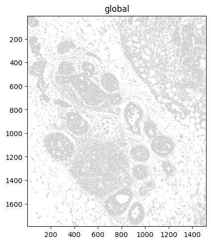
Let’s have a quick look at the data.

sdata.pl.render_shapes("cell_boundaries").pl.show()

Initialize SegTraQ objects

Next, we initialize a SegTraQ object. The reason for this is that different technologies call things differently: cell centroids could be called centroid_x, x_centroid, cell_x, … By initializing a SegTraQ object, we only have to tell SegTraQ where our data lives once.

Don’t worry if you do not know which parameters you need up front; just put in your spatialdata object (segtraq.SegTraQ(sdata)), and SegTraQ will tell you which arguments are wrong/missing.

st = segtraq.SegTraQ(
    sdata,
    images_key="image",  # where the image is stored
    tables_centroid_x_key="x_centroid",  # where the x centroid is stored
    tables_centroid_y_key="y_centroid",  # where the y centroid is stored
)

/g/huber/users/meyerben/notebooks/spatial_transcriptomics/SegTraQ/src/segtraq/SegTraQ.py:190: RuntimeWarning: Gene sets differ between assigned transcript points and the expression table. 0 genes occur only in points (e.g. []), and 6 occur only in the table (e.g. ['Human_CTNNB1_S33C_ALT:G', 'CYP2A6', 'Human_FGFR3_R248H_ALT:A', 'F2', 'Human_PTEN_G129E_WT:A']). Genes only occuring in the table can be introduced by cropping (`SpatialData`), but differences may also be due to the filtering used to generate the transcript data and expression matrix. Please check that `filter_kwargs`, particularly `min_qv` and `control_prefixes`, are consistent with the filtering used to generate the expression table.
  sdata_new = _filter_control_and_low_quality_transcripts(
/g/huber/users/meyerben/notebooks/spatial_transcriptomics/SegTraQ/src/segtraq/SegTraQ.py:190: RuntimeWarning: Cell IDs differ between assigned transcript points and the expression table. 0 cells occur only in points (e.g. []), and 50 occur only in the table (e.g. ['ibgnelbc-1', 'ipkonddj-1', 'ocnkohki-1', 'obnkiokn-1', 'japgdane-1']). Cells only occuring in the table can reflect zero-count cells, but differences may also be due to the filtering used to generate the transcript data and expression matrix. Please check that `filter_kwargs`, particularly `min_qv` and `control_prefixes`, are consistent with the filtering used to generate the expression table.
  sdata_new = _filter_control_and_low_quality_transcripts(

Now the data is ready to compute some quality control metrics. SegTraQ is structured into different modules, all of which focus on different problems that can arise during segmentation. We will now go through all of the modules and look at what they tell us about our segmentation.

Baseline module

The baseline (bl) module computes basic quality-control metrics such as the number of cells, the percentage of unassigned transcripts, and the number of transcripts and genes per cell. All of the results that SegTraQ computes are automatically stored in your spatialdata object.

# the number of cells
st.bl.num_cells()

18311

# the percentage of transcripts not assigned to any cell
st.bl.perc_unassigned_transcripts()

10.324546815309601

# the number of transcripts per cell
st.bl.transcripts_per_cell().head()

	cell_id	transcript_count
0	afbommff-1	1352
1	afbjnaja-1	1227
2	afbihifc-1	1216
3	afjdkagk-1	1105
4	aphbncjb-1	1072

# the number of genes per cell
st.bl.genes_per_cell().head()

	cell_id	gene_count
0	acceakgj-1	86
1	accebped-1	95
2	accedpdh-1	50
3	acceejoe-1	57
4	acceekkh-1	48

# the mean number of transcripts per gene per cell
st.bl.mean_transcripts_per_gene_per_cell().head()

	cell_id	mean_transcripts_per_gene
0	acceakgj-1	1.093023
1	accebped-1	1.147368
2	accedpdh-1	1.120000
3	acceejoe-1	1.140351
4	acceekkh-1	1.166667

We can also compute some morphological features of the cells using bl.morphological_features().

st.bl.morphological_features().head()

	cell_id	num_polygons	cell_area	perimeter	circularity	solidity	convexity	elongation	eccentricity	compactness
0	acceakgj-1	1	45.630318	25.596593	0.875183	0.974460	0.983536	1.097515	0.412076	14.358558
1	accebped-1	1	44.433013	25.224078	0.877577	0.969899	0.983684	1.377976	0.688009	14.319400
2	accedpdh-1	1	46.737367	26.267438	0.851214	0.964090	0.984115	1.367124	0.681882	14.762883
3	acceejoe-1	1	33.030204	22.242175	0.839009	0.968244	0.978508	1.214174	0.567164	14.977635
4	acceekkh-1	1	40.730569	23.923744	0.894277	0.982569	0.987680	1.117125	0.445754	14.051989

Clustering stability module

The clustering stability (cs) module provides metrics for assessing the stability of clustering results across different clustering resolutions and random subsets of genes. The idea is as follows: the better a segmentation method separates cell types, the better it is. We can compute a couple of metrics to investigate this.

Let`s first perform Leiden clustering and visualize the clusters in the UMAP space.

# extracting the anndata object from the spatialdata object and performing appropriate normalization
adata = st.sdata.tables["table"].copy()
sc.pp.normalize_total(adata, inplace=True)
sc.pp.log1p(adata)
sc.pp.pca(adata)
sc.pp.neighbors(adata)
sc.tl.umap(adata)
sc.tl.leiden(adata, flavor="igraph", n_iterations=2, resolution=0.2)

# plotting the result of the leiden clustering
sc.pl.umap(adata, color="leiden")

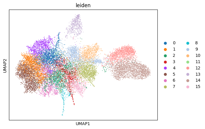
We can start by looking at the cluster connectedness. To compute it, we use the neighborhood graph we computed with scanpy earlier. The method then iterates over all cells and computes the number of neighbors with the same cluster assignment and divides it by the number of total neighbors. In general, the higher this value is, the better. By default, this is done at a resolution of 0.2, but you can adjust this with the resolution parameter.

st.cs.cluster_connectedness()

0.8205399021229313

We can do the same with the silhouette score.

st.cs.silhouette_score()

-0.03765101730823517

Next, we can check how stable the clustering is when we only take a subset (63%) of our genes and run clustering on this. We do this five times, and then assess the quality with the adjusted Rand index (ARI) and the purity. For more details on these metrics, refer to the section on this module.

st.cs.adjusted_rand_index()

0.6582868904489151

st.cs.purity()

0.7935927271283308

Region similarity module

The region similarity (rs) module evaluates morphological and molecular consistency across different regions of a cell. Transcript-based metrics are corrected for finite-count effects using permutation-based null expectations.

Matching nuclei to cells

match_nuclei_to_cells() matches each cell to its most overlapping nucleus. iou measures their overall overlap, while nucleus_fraction measures how much of the nucleus is contained within the cell.

st.rs.match_nuclei_to_cells().head()

	cell_id	nucleus_id	iou	nucleus_fraction	num_nuclei
0	acceakgj-1	0.0	0.617026	1.000000	1.0
1	accebped-1	1.0	0.556906	0.999997	1.0
2	accedpdh-1	2.0	0.427579	0.997749	1.0
3	acceejoe-1	3.0	0.708851	1.000000	1.0
4	acceekkh-1	4.0	0.543778	1.000000	1.0

Nucleus–cell similarity

similarity_nucleus_cell measures whether the final cell-level transcript profile is molecularly consistent with its matched nucleus. Negative residuals indicate lower similarity than expected.

st.rs.similarity_nucleus_cell().head()

	cell_id	nucleus_id	iou	nucleus_fraction	similarity_nucleus_cell	similarity_nucleus_cell_p_value
0	acceakgj-1	0.0	0.617026	1.000000	0.000147	0.542289
1	accebped-1	1.0	0.556906	0.999997	-0.030584	0.004975
2	accedpdh-1	2.0	0.427579	0.997749	-0.000677	0.532338
3	acceejoe-1	3.0	0.708851	1.000000	-0.014015	0.104478
4	acceekkh-1	4.0	0.543778	1.000000	-0.000529	0.472637

Nucleus–cytoplasm similarity

similarity_nucleus_cytoplasm directly compares nuclear and non-nuclear transcript composition. Low residuals may indicate transcript misassignment.

st.rs.similarity_nucleus_cytoplasm().head()

	cell_id	nucleus_id	iou	nucleus_fraction	similarity_nucleus_cytoplasm	similarity_nucleus_cytoplasm_p_value
0	acceakgj-1	0.0	0.617026	1.000000	-0.036996	0.119403
1	accebped-1	1.0	0.556906	0.999997	-0.102345	0.004975
2	accedpdh-1	2.0	0.427579	0.997749	-0.015371	0.388060
3	acceejoe-1	3.0	0.708851	1.000000	NaN	NaN
4	acceekkh-1	4.0	0.543778	1.000000	-0.129977	0.004975

Border admixture score

border_admixture_score asks whether the cell border resembles a mixture of the cell center and its neighborhood. Positive residuals indicate stronger neighborhood-like admixture than expected.

st.rs.border_admixture_score().head()

	cell_id	border_admixture_score	border_admixture_p_value
0	acceakgj-1	0.013326	0.378109
1	accebped-1	0.102202	0.094527
2	accedpdh-1	0.299454	0.019900
3	acceejoe-1	0.206444	0.009950
4	acceekkh-1	0.137160	0.054726

Supervised module

The sp (supervised) module provides metrics to evaluate how well cell profiles in a spatial transcriptomics dataset agree with a reference single-cell RNA-seq (scRNA-seq) dataset with cell type annotations.

Unlike scRNA-seq, contamination in spatial transcriptomics measurements mostly originates from the local tissue context.

By comparing spatial expression profiles to a high-quality scRNA-seq reference, the supervised module aims to quantify this mismatch. Specifically, we compute metrics that measure:

• how well each spatial cell matches its expected cell type,

• how much its expression resembles other (neighboring) cell types, and

• if it is possible to predict that a cell of one cell type is adjacent to a different cell type.

To obtain cell-type specific marker genes, we define positive and negative markers in the annotated scRNA-seq via markers_from_reference.

adata_ref = ad.read_h5ad("../../data/xenium_5K_data/BC_scRNAseq_Janesick.h5ad")

Computing cell-type specific markers

# hiding all warnings
with warnings.catch_warnings():
    warnings.simplefilter("ignore")

    markers = st.markers_from_reference(
        adata_ref,
        ref_cell_type="celltype_major",
        ref_raw_counts_layer="raw",
        n_jobs=16,
    )

WARNING: adata.X seems to be already log-transformed.

Below, we show the number of negative markers that overlap with the positive markers of each cell type. To reliably estimate contamination, each cell type should share at least ~5 negative markers with the positive marker set of every other cell type. If these overlaps are too small, contamination estimates become unstable.

In such cases, the marker definition can be relaxed by adjusting the thresholds used in markers_from_reference above.

ctypes = list(markers.keys())
overlap_df = pd.DataFrame(0, index=ctypes, columns=ctypes, dtype=int)

for c in ctypes:
    neg_c = set(markers[c].get("negative", []))
    for d in ctypes:
        pos_d = set(markers[d].get("positive", []))
        overlap_df.loc[c, d] = len(neg_c & pos_d)

overlap_df

	B	DCIS1	DCIS2	T	dendritic	endo	macro	mast	myoepi	perivas	stromal	tumor
B	0	49	39	26	50	108	71	28	97	87	98	22
DCIS1	50	0	16	48	66	90	76	27	33	49	70	16
DCIS2	48	20	0	52	63	92	74	29	58	60	84	6
T	41	75	78	0	73	110	102	37	98	109	118	66
dendritic	26	50	41	27	0	101	49	24	85	70	88	29
endo	44	37	27	37	49	0	60	24	55	6	31	22
macro	29	48	40	24	42	94	0	20	85	80	94	27
mast	47	50	56	43	70	86	74	0	70	92	109	38
myoepi	41	12	5	33	48	63	48	20	0	34	42	14
perivas	49	41	29	28	53	45	79	28	59	0	40	26
stromal	48	37	25	47	56	66	54	27	61	24	0	28
tumor	57	23	12	66	70	95	88	30	75	71	90	0

Label transfer

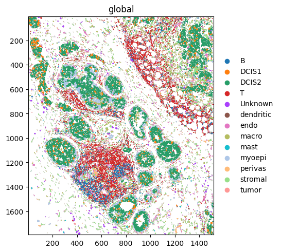
Before we can do statistics on the spatial data, we first need to transfer our cell type labels onto the spatial transcriptomics data. We can do this simply by calling run_label_transfer().

st.run_label_transfer(adata_ref, ref_cell_type="celltype_major", ref_raw_counts_layer="raw")

WARNING: adata.X seems to be already log-transformed.

Let’s quickly verify that this worked by plotting the data.

# Replace NaN with Unknown for plotting
s = st.sdata.tables["table"].obs["transferred_cell_type"]
if pd.api.types.is_categorical_dtype(s):
    s = s.cat.add_categories(["Unknown"])

st.sdata.tables["table"].obs["transferred_celltype_plot"] = s.fillna("Unknown")

# before we can plot, we need to link the shapes to the table
st.sdata.tables["table"].obs["region"] = "cell_boundaries"
st.sdata.set_table_annotates_spatialelement("table", region="cell_boundaries")

st.sdata.pl.render_shapes("cell_boundaries", color="transferred_celltype_plot").pl.show(coordinate_systems="global")

Marker purity

To quantify how well each segmented cell in the spatial transcriptomics data matches its annotated cell type, we defined a marker-based purity (marker_balanced_accuracy) score that jointly evaluates the expression of positive (positive_marker_recall) and the absence of neighborhood-associated negative markers (negative_marker_avoidance). The method accounts for the spatial context of each cell and is motivated by the assumption that differences between scRNA-seq and spatial transcriptomics-derived cell type profiles arise mainly from local contamination by neighboring cells.

st.sp.marker_purity(cell_type_key="transferred_cell_type", markers=markers).head()

INFO     Creating graph using `None` transform and `1` libraries.

	cell_id	positive_marker_recall	negative_marker_avoidance	marker_balanced_accuracy	n_evaluated_positive_markers	n_evaluated_negative_markers
0	acceakgj-1	0.062500	1.0	0.531250	112	4
1	accebped-1	0.071429	1.0	0.535714	112	5
2	accedpdh-1	0.016949	1.0	0.508475	118	5
3	acceejoe-1	0.062500	1.0	0.531250	112	5
4	acceekkh-1	0.062500	1.0	0.531250	112	17

These metrics are most informative when considered jointly. For an example, please refer to the Xenium Focus.

Neighborhood contamination

Marker purity summarizes how well a cell matches its own markers and avoids neighborhood-relevant negatives. In many cases, we also want to quantify

1. how many contaminating transcripts are present per cell and

2. which neighboring cell types contribute to this signal. We therefore compute neighborhood contamination.

per_cell_df, _, _, _ = st.sp.neighbor_contamination(cell_type_key="transferred_cell_type", markers=markers)
per_cell_df.head()

	cell_id	contamination_counts	contamination_strength
0	acceakgj-1	0.0	0.0
1	accebped-1	0.0	0.0
2	accedpdh-1	0.0	0.0
3	acceejoe-1	0.0	0.0
4	acceekkh-1	0.0	0.0

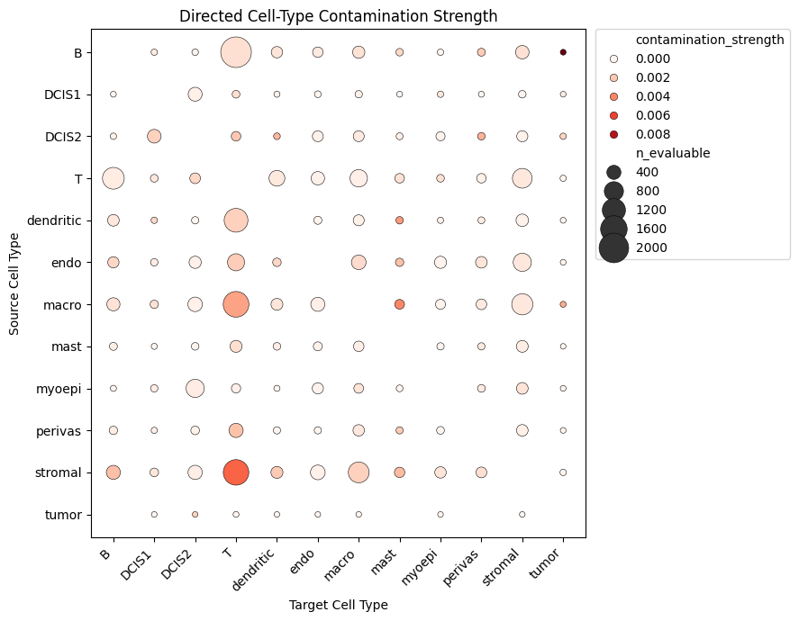
The heatmap below summarizes contamination strength for each source–target cell-type pair. Each entry represents the mean contamination strength across all evaluable target cells of the given target cell type, where the source-specific contamination strength is computed as the fraction of transcripts in the target cell that correspond to contamination-relevant markers of the source cell type.

The bubble plot illustrates the contamination strength (bubble color) and the number of evaluable target cells (bubble size). The number of evaluable cells depends on

1. how frequently the source and target cell types occur as neighbors and

2. how distinct their expression profiles are, as more transcriptionally distinct cell types have more mutually exclusive marker genes that can be evaluated.

Stromal cells cause a high level of contamination into neighboring cells.

cont_strength_mat = st.sdata.tables[st.tables_key].uns["contamination_strength_matrix"]
cont_n = st.sdata.tables[st.tables_key].uns["contamination_evaluable_cells_matrix"]

plot_df = (
    cont_strength_mat.stack(dropna=False)
    .rename("contamination_strength")
    .reset_index()
    .rename(columns={"level_0": "source", "level_1": "target"})
)

plot_df["n_evaluable"] = cont_n.stack(dropna=False).values

plt.figure(figsize=(9, 7))

ax = sns.scatterplot(
    data=plot_df,
    x="target",
    y="source",
    size="n_evaluable",
    hue="contamination_strength",
    sizes=(20, 600),
    palette="Reds",
    edgecolor="black",
)

ax.legend(
    bbox_to_anchor=(1.02, 1),
    loc="upper left",
    borderaxespad=0,
)

plt.title("Directed Cell-Type Contamination Strength")
plt.xlabel("Target Cell Type")
plt.ylabel("Source Cell Type")
plt.xticks(rotation=45, ha="right")
plt.tight_layout()
plt.show()

Mutually exclusive co-expression rate (MECR)

The mutually exclusive co-expression rate (MECR) is a measure for whether combinations of positive and negative markers (computed with a more stringent setting to increase mutual exclusivity, vote_frac_pos=0.3) co-occur less often than expected under independence.

tbl = st.sdata["table"]
common_genes = tbl.var_names[tbl.var_names.isin(adata_ref.var_names)]
adata_ref = adata_ref[:, common_genes].copy()

markers = st.markers_from_reference(
    adata_ref,
    ref_cell_type="celltype_major",
    ref_raw_counts_layer="raw",
    mode="de",
    min_pos_frac=0.3,
    n_jobs=16,
)

st.sp.mutually_exclusive_coexpression_rate(markers=markers).head()

WARNING: adata.X seems to be already log-transformed.

	gene1	gene2	odds_ratio	pvalue	a	b	c	d
0	IL3RA	TRBC1	0.424552	0.001375	11	236	1787	16277
1	NLRP1	TRIM29	0.438054	0.094415	3	420	287	17601
2	ITGA2B	SLC2A1	3.632042	0.993404	4	31	627	17649
3	CYP27A1	HES4	8.606262	0.998063	2	136	31	18142
4	PDGFRB	PSD3	2.154061	0.980095	7	368	157	17779

3D Volume Module

The volume (vl) accessor provides metrics to assess how well a segmentation method resolves cell overlaps in 3D. Spatial transcriptomics tissue sections have a finite thickness (~4–10 µm), so cells can overlap along the z-dimension and 2D segmentation methods may introduce mixing by assigning transcripts from overlapping cells to the same mask. In this module, we introduce metrics to quantify sensitivity to 3D overlap and evaluate how well quasi-3D methods (e.g. Proseg) disentangle transcripts from overlapping cells.

For a detailed description of this module, please refer to this tutorial.

Top–bottom z consistency

similarity_top_bottom compares transcript composition at the top and bottom of each cell to detect potential mixing from overlapping cells across z. Negative residuals indicate lower top–bottom similarity than expected, which may suggest overlapping or incorrectly merged cells.

st.vl.similarity_top_bottom().head()

	cell_id	similarity_top_bottom	similarity_top_bottom_p_value
0	acceakgj-1	-0.009827	0.189055
1	accebped-1	-0.124454	0.004975
2	accedpdh-1	0.038066	0.696517
3	acceejoe-1	-0.165040	0.009950
4	acceekkh-1	-0.185124	0.004975

In volume.ipynb, we explore the distribution of transcripts along the z-dimension in more depth and put it into context with ovrlpy, a package for detecting 3D overlap in spatial transcriptomics. There, we use a Xenium v1 dataset with a 313-gene panel, where transcript coverage is higher and the analysis is less affected by sparsity.

Point statistic metrics

The point statistics (ps) module is designed to compare the distribution of a set of transcripts in the cell relative to its cell centroid or cell border. The idea is to compute the distances of the transcripts to a reference point in the cell, either the cell centroid or the cell boundaries and aggregate this measure per transcript id.

Distance of transcripts to the cell membrane

In this metric we compute the distance to the segmented cell membrane of each transcript coordinate and aggregate this metric per transcript id as mean. For example, we can compute both the average distance to the cell membrane across all previously defined negative and positive markers for the cell type “DCIS2”.

border_distance_negative = st.ps.distance_to_membrane(
    markers["DCIS2"]["negative"],
    cell_type_key="transferred_celltype_plot",
    cell_type_query=["DCIS2"],
    inplace=False,
)

border_distance_positive = st.ps.distance_to_membrane(
    markers["DCIS2"]["positive"],
    cell_type_key="transferred_celltype_plot",
    cell_type_query=["DCIS2"],
    inplace=False,
)

border_distance_negative.head()

	cell_id	distance_to_cell_membrane_199_genes	cell_area	distance_to_cell_membrane_norm_199_genes
0	aeldpbbo-1	2.507427	176.880632	0.188533
1	hjbdpmpc-1	1.811994	262.673512	0.111802
2	hjbcgooh-1	1.801255	102.683823	0.177756
3	aeldbffd-1	1.841093	135.493824	0.158167
4	hjbddfam-1	3.342148	303.922122	0.191710

border_distance_positive.head()

	cell_id	distance_to_cell_membrane_70_genes	cell_area	distance_to_cell_membrane_norm_70_genes
0	hjbbcfmf-1	1.899841	173.102552	0.144399
1	hjappign-1	1.342379	66.878803	0.164146
2	aelekoij-1	2.000107	227.247765	0.132679
3	aelggapo-1	2.306222	253.712191	0.144787
4	hjbancln-1	2.751999	154.525538	0.221385

Session Info

print(sd.__version__)  # spatialdata
print(spatialdata_plot.__version__)

0.8.0
0.4.0