Module: Plotting#

One of the main usecases of SegTraQ is to compare different segmentation methods. To facilitate this task, you can make use of the plotting module (pl). In order to use it, you need to prepare your data in the form of a dictionary that maps the method name to the corresponding SegTraQ object.

To follow along with this tutorial, you can download the data from here.

Data Preparation#

First, we need to get the data into the right format. This closely follows the Xenium Focus.

[1]:

%load_ext autoreload
%autoreload 2

import warnings

import anndata as ad
import matplotlib.pyplot as plt
import scanpy as sc
import spatialdata as sd
import spatialdata_plot  # noqa

import segtraq

warnings.filterwarnings(action="ignore")

/g/huber/users/meyerben/notebooks/spatial_transcriptomics/SegTraQ/.venv/lib/python3.13/site-packages/scanpy/_utils/__init__.py:33: FutureWarning: `__version__` is deprecated, use `importlib.metadata.version('anndata')` instead.
  from anndata import __version__ as anndata_version
/g/huber/users/meyerben/notebooks/spatial_transcriptomics/SegTraQ/.venv/lib/python3.13/site-packages/scanpy/__init__.py:24: FutureWarning: `__version__` is deprecated, use `importlib.metadata.version('anndata')` instead.
  if Version(anndata.__version__) >= Version("0.11.0rc2"):
/g/huber/users/meyerben/notebooks/spatial_transcriptomics/SegTraQ/.venv/lib/python3.13/site-packages/scanpy/readwrite.py:16: FutureWarning: `__version__` is deprecated, use `importlib.metadata.version('anndata')` instead.
  if Version(anndata.__version__) >= Version("0.11.0rc2"):
/g/huber/users/meyerben/notebooks/spatial_transcriptomics/SegTraQ/.venv/lib/python3.13/site-packages/spatialdata/_core/query/relational_query.py:531: FutureWarning: functools.partial will be a method descriptor in future Python versions; wrap it in enum.member() if you want to preserve the old behavior
  left = partial(_left_join_spatialelement_table)
/g/huber/users/meyerben/notebooks/spatial_transcriptomics/SegTraQ/.venv/lib/python3.13/site-packages/spatialdata/_core/query/relational_query.py:532: FutureWarning: functools.partial will be a method descriptor in future Python versions; wrap it in enum.member() if you want to preserve the old behavior
  left_exclusive = partial(_left_exclusive_join_spatialelement_table)
/g/huber/users/meyerben/notebooks/spatial_transcriptomics/SegTraQ/.venv/lib/python3.13/site-packages/spatialdata/_core/query/relational_query.py:533: FutureWarning: functools.partial will be a method descriptor in future Python versions; wrap it in enum.member() if you want to preserve the old behavior
  inner = partial(_inner_join_spatialelement_table)
/g/huber/users/meyerben/notebooks/spatial_transcriptomics/SegTraQ/.venv/lib/python3.13/site-packages/spatialdata/_core/query/relational_query.py:534: FutureWarning: functools.partial will be a method descriptor in future Python versions; wrap it in enum.member() if you want to preserve the old behavior
  right = partial(_right_join_spatialelement_table)
/g/huber/users/meyerben/notebooks/spatial_transcriptomics/SegTraQ/.venv/lib/python3.13/site-packages/spatialdata/_core/query/relational_query.py:535: FutureWarning: functools.partial will be a method descriptor in future Python versions; wrap it in enum.member() if you want to preserve the old behavior
  right_exclusive = partial(_right_exclusive_join_spatialelement_table)

[2]:

# === READING SPATIALDATA OBJECTS ===
sdata_xenium_ws = sd.read_zarr("../../data/xenium_5K_data/xenium.zarr")
sdata_bidcell_ws = sd.read_zarr("../../data/xenium_5K_data/bidcell.zarr")
sdata_proseg_ws = sd.read_zarr("../../data/xenium_5K_data/proseg2.zarr")
sdata_segger_ws = sd.read_zarr("../../data/xenium_5K_data/segger.zarr")

# === CROPPING ===
bb_xmin = 800
bb_ymin = 1150
bb_w = 200
bb_h = 300
bb_xmax = bb_xmin + bb_w
bb_ymax = bb_ymin + bb_h


def crop(ws):
    return ws.query.bounding_box(
        axes=["x", "y"],
        min_coordinate=[bb_xmin, bb_ymin],
        max_coordinate=[bb_xmax, bb_ymax],
        target_coordinate_system="global",
    )


sdata_xenium = crop(sdata_xenium_ws)
sdata_bidcell = crop(sdata_bidcell_ws)
sdata_proseg = crop(sdata_proseg_ws)
sdata_segger = crop(sdata_segger_ws)

# === CREATING SEGTRAQ OBJECTS ===
st_xenium = segtraq.SegTraQ(
    sdata_xenium, images_key="image", tables_centroid_x_key="x_centroid", tables_centroid_y_key="y_centroid"
)
st_bidcell = segtraq.SegTraQ(
    sdata_bidcell,
    images_key="image",
    points_background_id=0,
    tables_centroid_x_key="centroid_x",
    tables_centroid_y_key="centroid_y",
)
st_proseg = segtraq.SegTraQ(
    sdata_proseg,
    images_key="image",
    points_background_id=0,
    tables_area_key=None,
    tables_centroid_x_key="centroid_x",
    tables_centroid_y_key="centroid_y",
)
st_segger = segtraq.SegTraQ(
    sdata_segger, images_key="image", tables_centroid_x_key="cell_centroid_x", tables_centroid_y_key="cell_centroid_y"
)

# === PUTTING EVERYTHING INTO A DICTIONARY ===
st_dict = {"xenium": st_xenium, "bidcell": st_bidcell, "proseg": st_proseg, "segger": st_segger}

# === REMOVING CONTROL PROBES ===
for method, st in st_dict.items():
    qv = 30 if method == "segger" else 20
    st.filter_control_and_low_quality_transcripts(min_qv=qv)

no parent found for <ome_zarr.reader.Label object at 0x7fc4a79cf380>: None
no parent found for <ome_zarr.reader.Label object at 0x7fc4a5050cd0>: None
no parent found for <ome_zarr.reader.Label object at 0x7fc4a5053610>: None
no parent found for <ome_zarr.reader.Label object at 0x7fc4a5056ea0>: None
no parent found for <ome_zarr.reader.Label object at 0x7fc4a7982060>: None
no parent found for <ome_zarr.reader.Label object at 0x7fc4a7a4dd90>: None
no parent found for <ome_zarr.reader.Label object at 0x7fc4a79c6f10>: None
no parent found for <ome_zarr.reader.Label object at 0x7fc4a79c7130>: None
no parent found for <ome_zarr.reader.Label object at 0x7fc4a5075a50>: None
no parent found for <ome_zarr.reader.Label object at 0x7fc4a5075d50>: None
no parent found for <ome_zarr.reader.Label object at 0x7fc49e36bd40>: None
no parent found for <ome_zarr.reader.Label object at 0x7fc49e36b020>: None

Run desired metrics#

Now, we can run all of the metrics we want on this dataset. For now, we simply run a label transfer and run some scanpy functions to compute the UMAP coordinates.

[3]:

# running computations for UMAP etc.
for _, st in st_dict.items():
    # extracting the anndata object from the spatialdata object and performing appropriate normalization
    adata = st.sdata.tables["table"]
    adata.layers["raw"] = adata.X.copy()
    sc.pp.normalize_total(adata, inplace=True)
    sc.pp.log1p(adata)
    sc.pp.pca(adata)
    sc.pp.neighbors(adata)
    sc.tl.umap(adata)

# Load scRNA-seq data
adata_ref = ad.read_h5ad("../../data/xenium_5K_data/BC_scRNAseq_Janesick.h5ad")

# Transfer labels
for _method, st in st_dict.items():
    st.run_label_transfer(
        adata_ref, ref_cell_type="celltype_major", inplace=True, ref_ensemble_key=None, query_ensemble_key=None
    )

Plots for individual samples#

The pl module provides methods to plot different things: on one hand, it can be used to visualize certain characteristics of a sample, and on the other, it can be used to compare between different samples or segmentation methods. Let’s start by looking at some sample-specific plots. Specifically, we can look at the distribution of transcripts and different segmentation features across the x and y coordinate. For some technologies (such as CosMx), this can help to detect stitching artefacts.

[4]:

# transcript distribution across the x and y axis of the image
# the smoothing factor (default: 10) can be used to get an idea for broader trends
_ = st_xenium.pl.transcript_distribution_across_space(smoothing=10)

[5]:

# features of the segmentation across the axes
_ = st_xenium.pl.feature_distribution_across_space(features=["cell_area", "nucleus_area"], smoothing=10)

We can see two things here: for the Xenium segmentation, the right part of the image contains more transcripts. Its cells are also larger. We can use spatialdata_plot to have a look at the actual data.

[16]:

fig, ax = plt.subplots(1, 2, figsize=(7, 7), dpi=100)
st_xenium.sdata.pl.render_points("transcripts", size=0.01, color="red", method="matplotlib").pl.show(ax=ax[0])
st_xenium.sdata.pl.render_shapes("cell_boundaries").pl.show(ax=ax[1])

Here, this is actually due to the structure of the tissue (large tumor cells are on the right side of the image). When applying these methods on larger tissues, they can also help to detect technical artefacts.

Comparing between segmentation methods#

We can also use the pl module to compare between different segmentation methods. All we need to do is pass our dictionary of SegTraQ objects.

[7]:

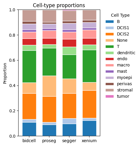
_ = segtraq.pl.celltype_proportions(st_dict, celltype_col="transferred_cell_type")

[8]:

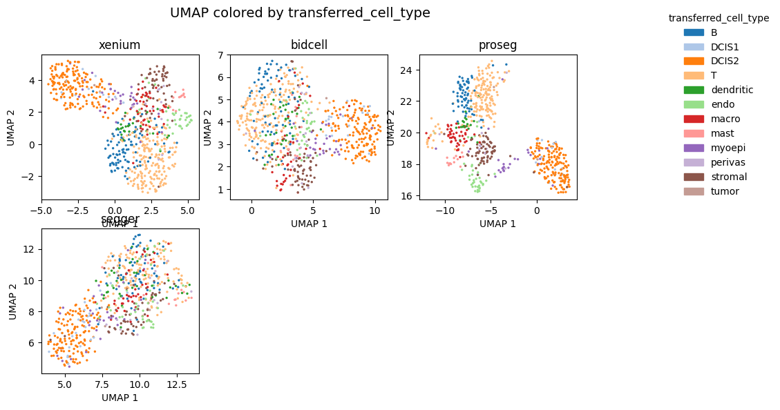
_ = segtraq.pl.umap(st_dict, color="transferred_cell_type", legend=True, figsize=(10, 6))

[9]:

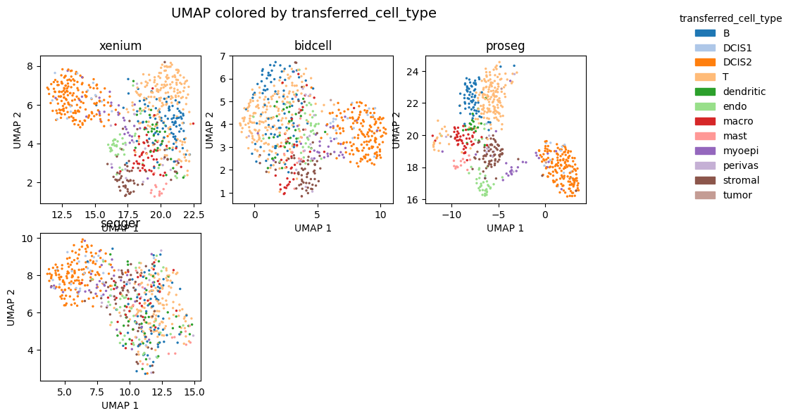
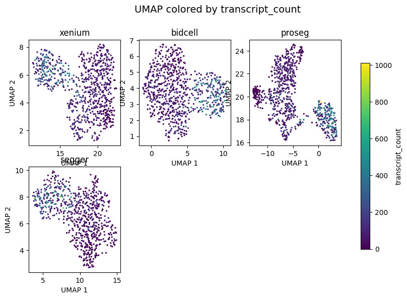
_ = segtraq.pl.umap(st_dict, color="transcript_count", legend=True, figsize=(10, 6))

[10]:

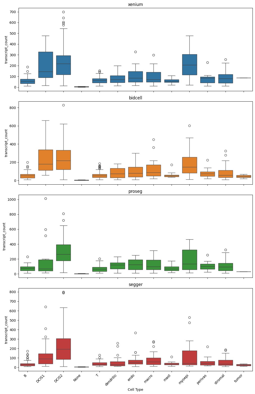
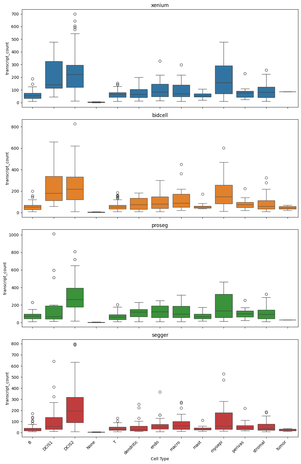
_ = segtraq.pl.boxplot(st_dict, celltype_col="transferred_cell_type", value_key="transcript_count")

[11]:

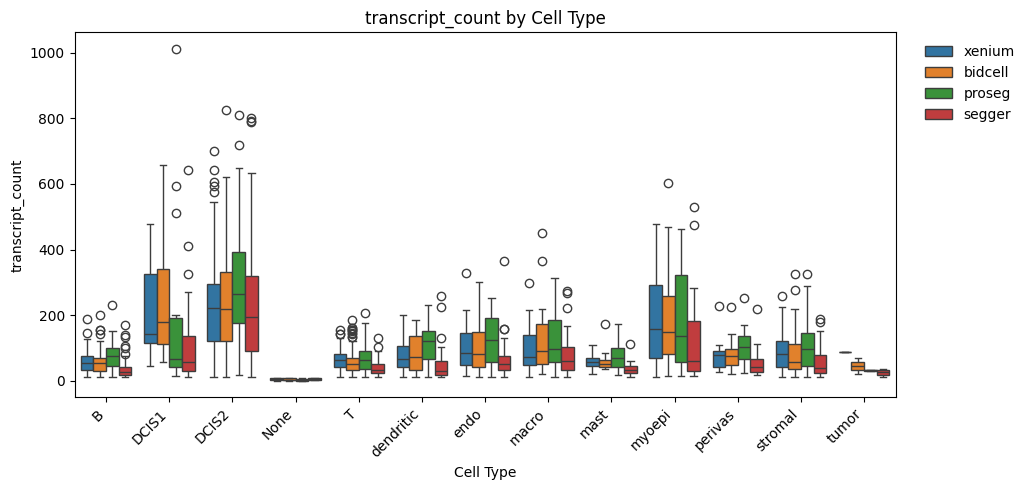
_ = segtraq.pl.boxplot_combined(st_dict, celltype_col="transferred_cell_type", value_key="transcript_count")

Session Info#

[12]:

print(sd.__version__)  # spatialdata
print(spatialdata_plot.__version__)

0.7.2
0.3.3

Module: Plotting

Contents